Using the the GCCBMC algorithm, several physical properites of polymeric systems were studied in this project. We studied the temperature and density effects on polymer conformation and the phase behavior of the polymer system. The efficiencies of the GCCBMC algorithm is also compared with an algorithm using reptation to move the polymers.
Our
first concern is to make sure that the simulation is working properly and
also to characterize the system. To do this, the radius
of gyration of the polymer (Rg) is measured at various chainlengths
(Nm) and temperature (T). Statistical theories of polymers4
predict that Rg ~ Nmv , where v is
a temperature - dependent coefficient due to competing intra-polymer and
inter-polymer interactions. Theories, experiments, and other simulations
have shown that at a theta temperature (T_theta), the polymer has an ideal
random walk conformation and v = 0.5. For T >T_theta, the
polymer has a self-avoiding walk conformation and v=0.6. For
T < T_theta, the polymer has a collapsed conformation and v =
0.33. The system used to study the polymer conformations in this
project has fixed volume, temperature, and only one polymer. The
polymer is allowed configurational-bias moves. The results of the
simulations done are shown in the following plot.
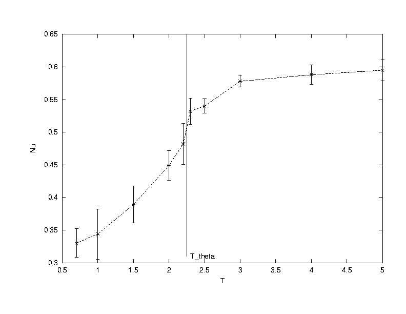
The exponent v is extracted from the simulations of a single polymer performing configuration moves in a NVT system of boxlength 100. By varying the number of monomer units (Nm) in the polymer from 4 to 64, the exponent is determined from curve fitting Rg vs Nm.(Click on the graph to get an enlarged view.)
Another
physical trend that we can check against is that the monomer - monomer
correlations between polymers should increase as the density of polymers
increase. The inter-polymer density correlation is defined as
.gif)
where V is the system
volume, N is the number of particles in the system, and rij
is the distance between particles i and j. The algorithm used to
calculate g(r) from the simulation data can be found here.
The inter-polymer density correlation function was calculated from the
simulations done at T = 4, boxlength = 12. 1000 MC steps was collected
after 2000 MC steps of equilibration. 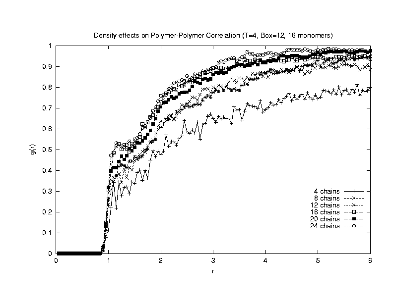
From the graph, it
can be concluded that the simulation does agree with the physical trend
of increasing correlation with increasing density. Also, at a higher
density of 0.22 (24 chains), a small peak at r = 1 can be observed.
This indicates that polymers are starting to form structures, and this
effect is more prounouced at higher densities, as shown in the following
plot.(Click on the graph to get an enlarged view.)
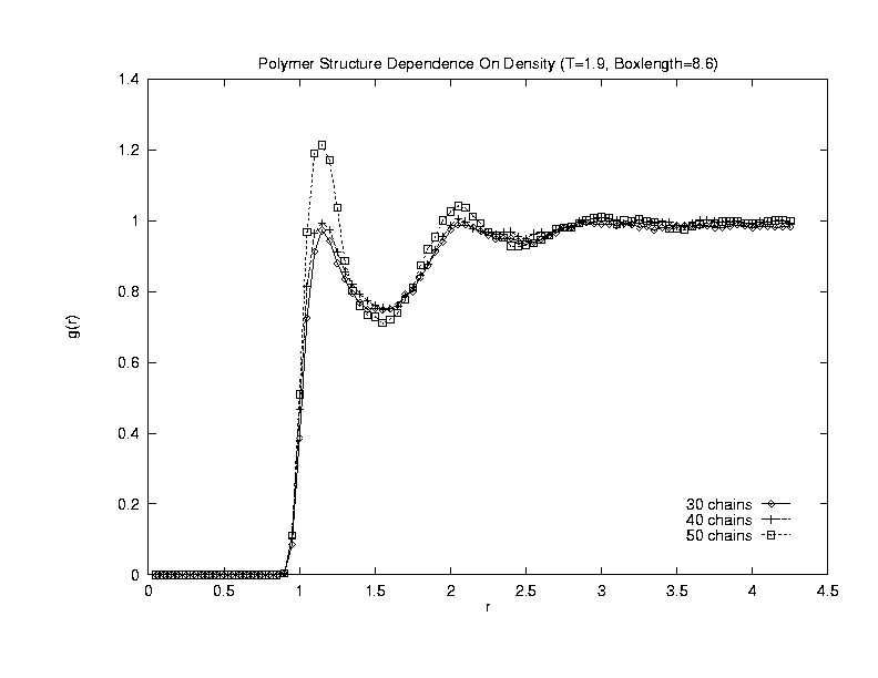
This plot shows a NVT system of boxlength 8.6 at T=1.9 containing 8-monomer chains. The peaks in the density-correlation functions are now prounced and indicate liquid shells of polymers forming in the system.(Click on the graph to get an enlarged view.)
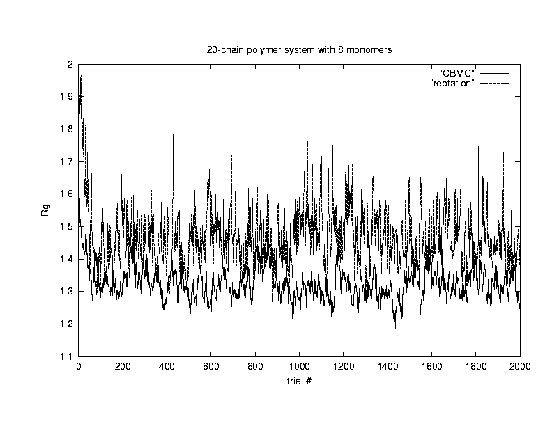
Our next concern is about the efficiency of the configurational - bias algorithm. Because polymers are molecules on chains, it is very difficult to move them around with random walk in a dense system using conventional Monte Carlo due to the low acceptance ratio. Algorithms such as reptation7, pivoting8, and configurational bias have been used by researchers to increase the acceptance ratio. In this project, we compared the efficiencies of the configurational bias method against that of the reptation method using Rg as the quantity of concern. Since efficiency ~ 1/ (error^2 * time), the error bars in Rg and computer time are determined from the simulation.
For this comparison,
we chose a system with 50 polymers, each polymer consists of 8 monomers.
The system is a cube with length 8.6 to a side, and the temperature is
chosen as 1.9. The density of this system is 50*8/(8.6)^3
= 0.63. The system is allowed to equilibrate for 2000 Monte Carlo
steps, then the data is sampled for 500 MC steps. The following plot
shows that using configuartional-bias algothrim allows faster equilibration
and also achieves better efficiency under these conditions.(Click on the graph to get an enlarged view.)
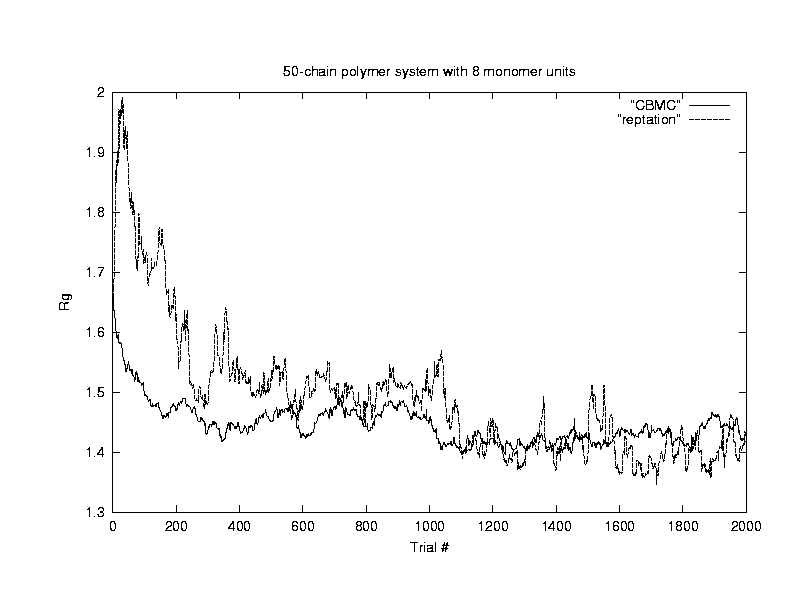
| time | Rg | sigma(Rg) | corr. time | efficiency | acc ratio (%) | |
| Reptation | 119.7 | 1.420 | 0.011 | 50 | 15.6 | 3.78 |
| CBMC(k=8) | 400.9 | 1.412 | 0.007 | 15 | 23.8 | 10.97 |