Dijkstra's Algorithm
by Siping MengOverview
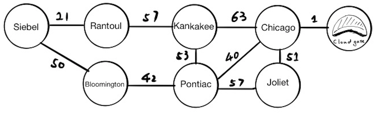
We know from mp_traversals that BFS can be used to find the shortest path between two points. So why Dijkstra’s algorithm? Besides their different time and space complexities, BFS can only be used on an undirected graph, such as a maze. However, Dijkstra’s algorithm can be used on weighted edges. For example, if you want to find the shortest driving path from Siebel Center to the Cloud Gate located in downtown Chicago, you have to think about how long you need to drive for each road. The edge weights are the time you need to spend on the roads (under the speed limit). In this note, we will assume all the roads between Siebel and the Cloud Gate are the same, and there are no traffic jams.
In this problem, each node represents the city we may travel to, and each edge represents the time(in minutes) traveling between two cities. The starting node is “Siebel,” the destination node is “Cloud Gate.”
Algorithm
What we need?
Before running the Dijkstra’s algorithm, we need to set up an visited set and a tentative distance value for each node.
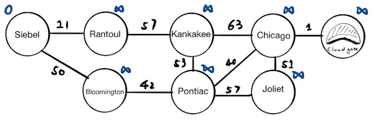
Firstly, we set the tentative distance value for starting node(Siebel) to 0 and all other nodes to infinity. The tentative distance means the up-to-date distance between this node to the starting node. Since we are not exploring yet, everything other than the starting node is set to infinity.
Secondly, we have an empty visited set now because we have not yet visited any node. To visualize this set on the graph, we will use the red color.
Thirdly, we need a priority queue to find the next closest unvisited node. Each item inside the queue contains two elements: the node and its tentative distance value. If we pop everything from the priority queue now, we will get:
[(“Siebel”, 0)]
Run Dijkstra’s algorithm
We will keep traversing the neighbors of the nodes that are at the top of the priority queue. For each neighbor, we will:
- Update the neighbor’s tentative distance value if we found a closer path.
- Put the neighbor into the priority queue.
- Put the current node into the visited set.
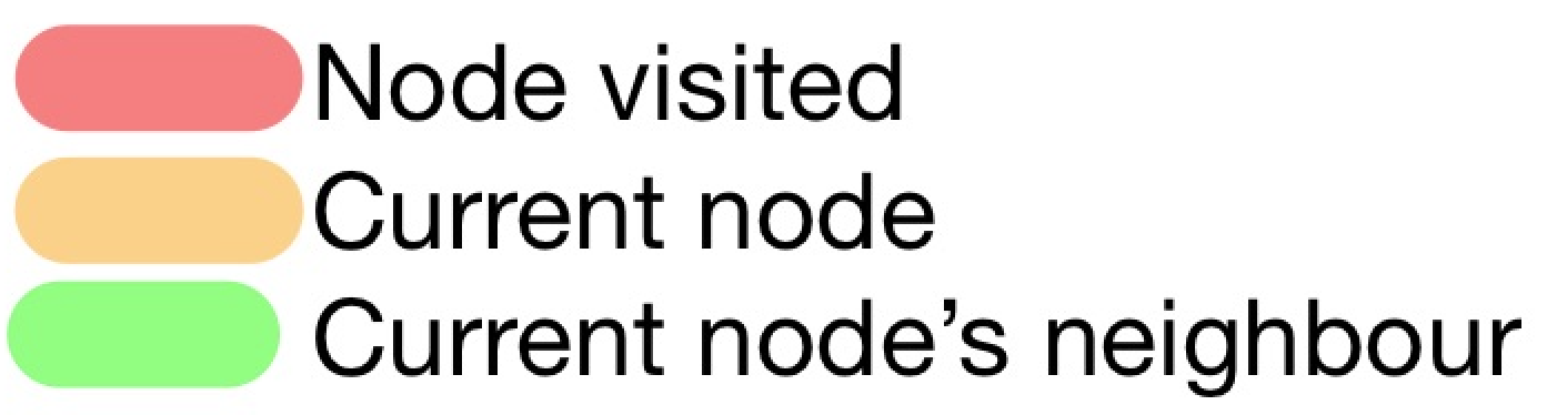
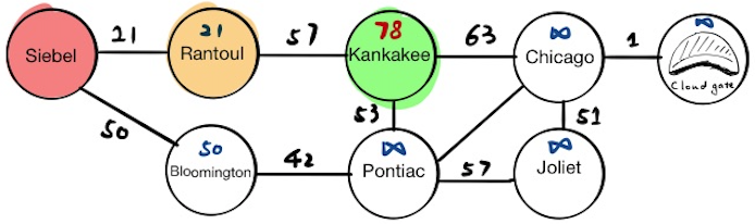
This is the legend for how we are going to traverse this graph.
Siebel
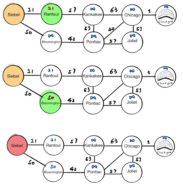
The first stop is Siebel, which has two neighbors, Rantoul and Bloomington. We will update their tentative distance values respectively and push the results into the priority queue. If we pop everything from the priority queue now, we will get:
[(“Rantoul”, 21), (“Bloomington”, 50)]
Finally, we mark Siebel as visited.
Rantoul
Since Rantoul is at the top of the priority queue, the current node will become Rantoul. We will update the tentative distance value for Rantoul’s neighbors, and if we pop everything from the priority queue now, we will get:
[(“Bloomington”, 50), (“Kankakee”, 78)]
Finally, we mark Rantoul as visited.
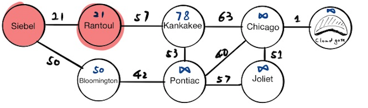
Bloomington
Now Bloomington is at the top of the priority queue, and the current node will become Bloomington. We will update the tentative distance value for Bloomington’s neighbors, and if we pop everything from the priority queue now, we will get:
[(“Kankakee”, 78), (“Pontiac”, 90)]
Finally, we mark Bloomington as visited.
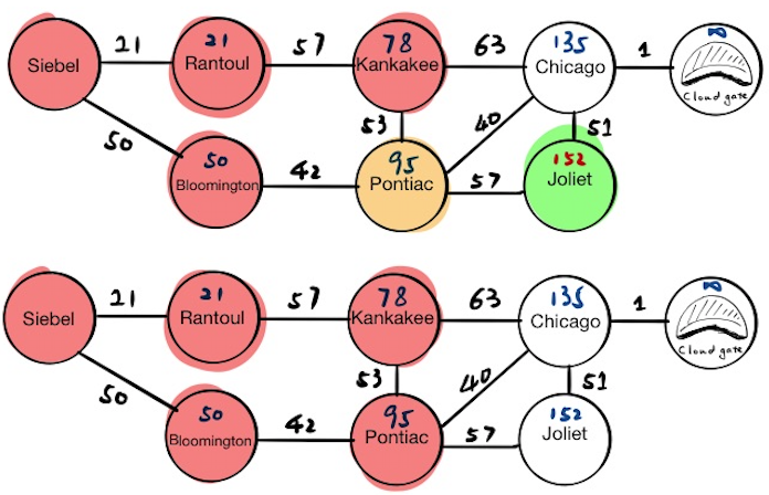
Kankakee
Now Kankakee is at the top of the priority queue, and the current node will become Kankakee. We will update the tentative distance value for Kankakee’s neighbors, and if we pop everything from the priority queue now, we will get:
[(“Pontiac”, 90), (“Chicago”, 141)]
Finally, we mark Kankakee as visited.
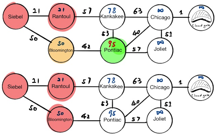
Pontiac
Now Pontiac is at the top of the priority queue, and the current node will become Pontiac. We will update the tentative distance value for Pontiac’s neighbors. In this step, notice that we have overwritten Chicago’s tentative distance value because we find a shorter path. If we pop everything from the priority queue now, we will get:
[(“Chicago”, 135), (“Joliet”, 152)]
Finally, we mark Pontiac as visited.
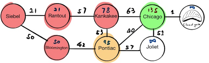
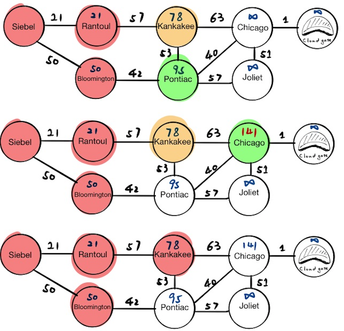
Chicago
Now Chicago is at the top of priority queue, the current node will become Chicago. We will update the tentative distance value for Chicago’s neighbors and if we pop everything from the priority queue now, we will get:
[(“Cloud Gate”, 136), (“Joliet”, 152)]
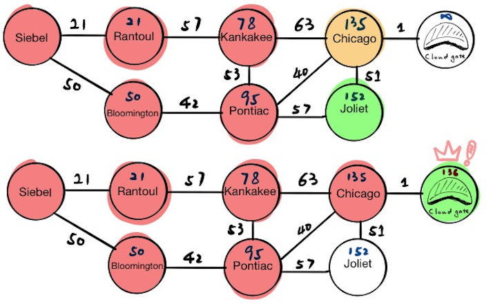
Cloud Gate
The algorithm finishes because this is the destination.
Psedocode
Dijkstra(Graph, source, destination):

  initialize distances  // initialize tentative distance value
  initialize previous   // initialize a map that maps current node -> its previous node
  initialize priority_queue   // initialize the priority queue
  initialize visited

  while the top of priority_queue is not destination:
      get the current_node from priority_queue
      for neighbor in current_node's neighbors and not in visited:
          if update its neighbor's distances:
              previous[neighbor] = current_node
      save current_node into visited

  extract path from previous
  return path and distance
Complexity
- Each edge is viewed at most 2 times
- Each node is viewed at most twice: once for adding it to the queue, and a second for querying. If we use a heap for the priority queue (e.g. binary heap), it takes constant time to queue the node and logarithmic time to query the node
Total runtime: