Results

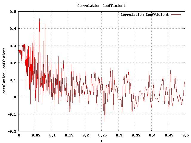
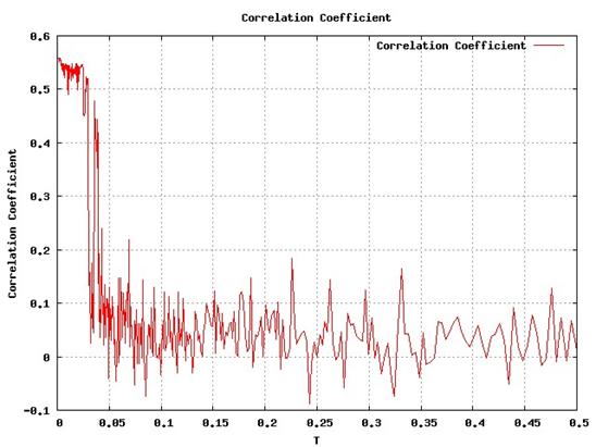
The temperature is defined by the scale of the correlation coefficient. We therefore choose T_0 = 0.5 and T_min = 0.001. Since we wanted to explore phase space a much as possible we chose dm=2000, ds =1000 and dphi=1.0. In addition we chose nstep=100 to guarantee a certain speed. Using these values a typical result for a run is shown in figure (cc_stop_0) for the image stop_0:

 

 

 

 

 

 

 

 

 

 

 

 

 

 

 

 

 

 

 

 

 

 

 

 

 

 

 

 

 

 

 

 

 

 

 

 

 

 

 

 

 

 

 

 

 

 

 

The correlation coefficient is shown below for figure cc_dne_5, and one can see that, although a larger maximum was found the simulation ends at a lower value.

 

 

 

 

 

 

 

 

 

 

 

 

 

 

 

Correlation Coefficient for stop_0 image with: nstep=100, dm=2000, ds=1000, dphi=1, tfactor=0.99. In addition the global maximum found coincides with the last state.

Best found matches for the run mentioned above

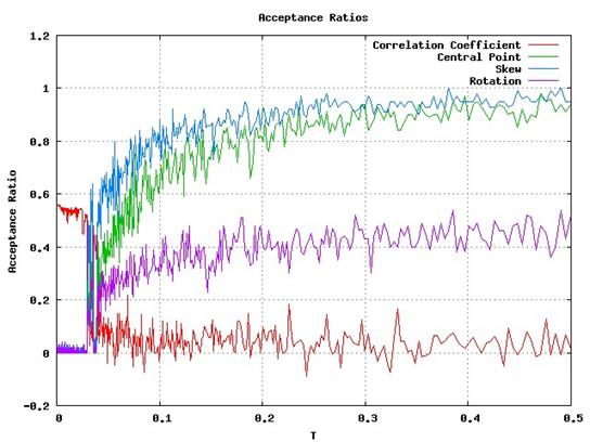
The acceptance ratios are shown in figure (ratio_stop_0). As one can see the maximum correlation is reached when the ratios are dropping. 

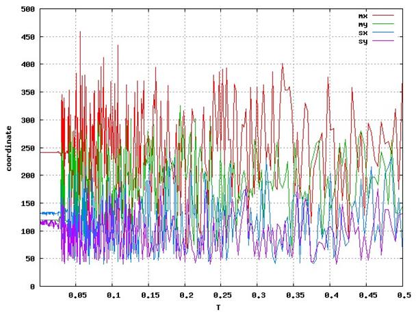
The trace of the actual values  is shown below:

Unfortunately the best match was not always the last match. In fact a big problem was that the search got stuck in a local maximum.

Best match

Last match

Summarizing the run mentioned above we obtained the following result

The maximal correlations are highlighted. As one can see for the images with a do-not-enter (dne_2) sign, the algorithm finds the sign. The first value however is suspicious since the correlation of 0.3801 is very low. The same holds true for the no-turn-on-right sign (ntor_2).

In contrast the correlations found for dne_5 and stop_0 are high.

 

 

In order to improve the algorithm one has to consider the acceptance ratios. As shown above, the ratios are almost one until T=0.05.  The initial temperature was therefore changed to T0 =0.05 and more Monte-Carlo steps were considered (nstep=1000). We obtained the following results:

 

Since the matching results were not satisfying we calculated the number of coherence cells of our model pictures. The number of coherence cells is defined as:

 

 

 

 

 

 

 

 

 

 

 

 

 

 

 

The number of coherence cells can be interpreted as the number of degrees of freedom of the template. A high number should result into robust recognition.

 

 

The following tables shows a summary of the number of coherence cells of our models:

Copyright 2010.

All rights reserved.

Evolution and Simulated Annealing

We started with 100 individuals, thermalized the system and reduced the number of individuals by a factor 2 each step until only 5 individuals were left.

We obtained the following results:

 

 

As one can see, the algorithm performs worse than the simple Simulated Annealing.

However we suspect that this approach has high potential, since due to lack of time it was not possible to determine the right selecting –rate.