Summary of Computer Simulations

Charged Particles

---

Introduction and Overview

This set of simulations adds charge to the gold particles and observes the results. Note that this experiment has not been conducted before in a labratory, so there are no experimental results to compare with in this case.

This set of simulations involved placing particles randomly on a 500 × 500 lattice, each with a charge of +1.6e-19 Coulombs, or -1.6e-19 Coulombs. The net charge of the system is zero. That is, the number of particles placed was always even, and half were always positively charged, while the other half were always negatively charged.

When clusters form, the net charge of the cluster is set equal to the sum of the charges held by the atoms forming that cluster. For example, two atoms with a positive charge of one would form a cluster with a positive charge of two. An cluster with a positive charge of two merging with a cluster with a negative charge of two would form a cluster of zero charge, that would then interact with other particles only through a Lennard-Jones potential, and not a Coulomb potential.

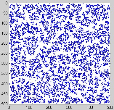
Images

The following image shows a typical end configuration.

Simulations and Results

The following simulations were run to determine the relation between the average cluster size, the number of clusters, and the simulation time:

1. A 500x500 system of 52,500 atoms (21% coverage).
2. A 500x500 system of 47,500 atoms (19% coverage).
3. A 500x500 system of 27,500 atoms (11% coverage).

A sample plot of the average cluster size vs. the simulation time is shown below.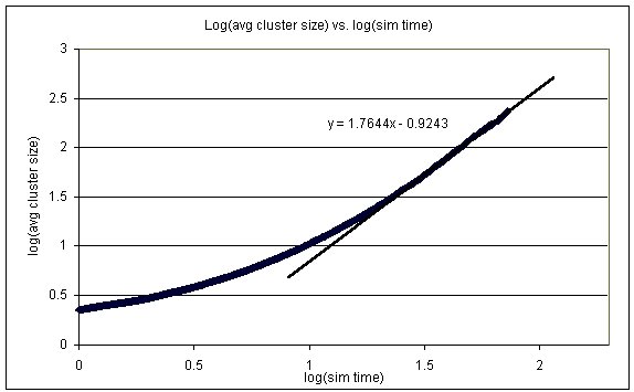 

A sample plot of the number of clusters vs. the simulation time is shown below. 

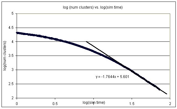
Note that for our simulation, as the number of particles is conserved, the average cluster size and the total number of clusters are not independent variables. As such, our slopes (tabulated below) will have the same error bars, and will differ only by a sign. In the experimental case, these two variables are not independent, so we have compared our (dependent) results to their (independent) results for the sake of completeness.

The following data was observed:

Coverage	Slope of log(avg cluster size) vs. log(sim time)	Experimental Results
21%	1.98 +/- 0.02	Unknown
19%	1.76 +/- 0.01
11%	1.50+/- 0.00

Coverage	Slope of log(#clusters) vs. log(sim time)	Experimental Results
21%	-1.98 +/- 0.02	Unknown
19%	-1.76 +/- 0.01
11%	-1.50+/- 0.00

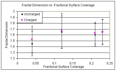
The following simulations were run to estimate the average fractal dimension for various coverage densities:

4. A 500x500 system of 10,000 atoms (4% coverage)
5. A 500x500 system of 30,000 atoms (12% coverage).
6. A 500x500 system of 52,500 atoms (21% coverage).
7. A 500x500 system of 57,500 atoms (23% coverage).

The following data was observed:

For simulation #4 :

Average fractal dimension computed to be 1.522 +/- 0.227.

For simulation #5 :

Average fractal dimension computed to be 1.67 +/- 0.3.

For simulation #6 :

Average fractal dimension computed to be 1.632 +/- 0.187.

For simulation #7 :

Average fractal dimension computed to be 1.645 +/- 0.215.