Thermal Conductivity of Argon from the Green-Kubo Method

Kim Seng Cheong

Xuan Zheng

 

Abstract

In this class project, we estimate the thermal conductivity of solid Argon using the fluctuation-dissipation theorem of Green-Kubo. Separate codes were written to simulate Argon in both the NVT and NPT ensembles. The Lennard-Jones 6-12 potential is used to model the atomic dynamics. Verlet neighbour lists are used to speed up the computation. We find good agreement with experimental data (~30%). Finite size effects are found to be negligible. The Green-Kubo formalism is hence found to be suitable for the determination of thermal conductivity in solids, contrary to previous studies.

Overview

This report is divided into the following sections:

• Motivation
• Introduction
• Methods & Results
• NVT
• NPT
• Summary
• References
• Source Codes
• Presentation

Motivation

Previous simulations of thermal conductivity of solid Argon in 1999 (Kaburaki et. al) yielded a factor of 2 discrepancy with experimental results. It was postulated that the Lennard-Jones 6-12 pair potential does not describe the atomic interactions of solid Argon well. This is unexpected as the LJ potential has been proven to be reliable in predicting both static and dynamical properties of both solid and fluid Argon. However, in a recent study by Tretiakov (2004), he reported a 20% discrepancy with experimental values. This agrees with the results of LJ fluids, which have a 10 % discrepancy with experiment in a wide temperature range (Vogelsang et al.). Due in part to the conflicting simulation results presented in literature as well as reports of the similar discrepancies in the calculation of thermal conductivity of other solids (Jund et al.), we were motivated to determine the following:

 

·        Whether the LJ parametrization of Argon is valid for the solid phase

·        Whether the Green-Kubo approach is valid for the determination of thermal conductivity in solids

 

Argon at high temperature is well described by hard sphere interactions (LJ) which can be determined via a cheap pairwise computation of the forces, as opposed to other more accurate, but more expensive potentials. This is important because the Green-Kubo method requires long run times (>10⁶ time steps) for good statistics. A simple potential also allows us to investigate finite size effects since the computation time scales quadratically with system size.

Introduction

The Lennard Jones system has been widely used as a model potential for rare gas interactions. The pair potential can be written as:

                           (1)

 

Where  is the distance between atoms i and j. This simple potential has been found to describe the classical behaviour of molecules with simple van der Waals attraction well. A typical LJ potential curve is shown below.

Fig. 1 A typical Lennard-Jones potential curve.

 

For Argon, the values of the parameters  and  that best reproduce its thermodynamics are  and .

 

Solid Argon crystallizes in an FCC configuration as shown below. The yellow box indicates 1 unit cell.

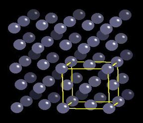
Fig. 2 A schematic diagram of an FCC lattice.

 

The FCC lattice is generated for box sizes ranging from 3-7 unit cells in our study. Initial velocities are assigned according to the Maxwell-Boltzmann distribution. The density is set to approximately 1 as reported in literature for the range of P/T under study. The temperature range studied is 10-70 K.

Thermal conductivity is defined as the linear coefficient relating the macroscopic heat current to the temperature gradient (Fourier’s law):

                                                (2)

 

In this project, we calculate  using the Green-Kubo formula:

                        (3)

 

Where V is the volume and T is the temperature. Angular brackets denote the average over time. The factor 3 is to account for averaging over the 3 dimensions. The microscopic heat current is given by:

        (4)

 

Where is the velocity of particle i and  is the force on atom i due to its neighbour j from the LJ potential. The site energy  is given by:

                           (5)

 

The Green-Kubo formalism allows us to calculate many dynamical properties such as viscosity, thermal conductivity and electrical conductivity from equilibrium simulations of atomic systems, as opposed to non equilibrium molecular dynamics (NEMD). Either way, calculations of  generally require large cells and long time scales to converge the statistical sampling. As a consequence, the thermal conductivity of real materials has been calculated so far only for a restricted set of substances and at best with a semi-empirical description of the interatomic interactions.

 

Error is estimated by the autocorrelation time of the microscopic heat current, after making the simplifying assumption that Gaussian statistics apply:

                    (6)

 

NVT Ensemble – Methods & Results

Argon atoms were put into an FCC lattice and assigned with velocities from a Gaussian distribution. Then a Verlet neighbor list was generated. Since the system is solid during simulations, we did not update the neighbor list during the run. The potential we used is the Lennard-Jones potential. We use Verlet algorithm to integrate the equation of motion. The time step is 0.002 reduced units. We quench the system to the desired temperature every 100 steps, and repeated for 100 times. After this, no thermostat is applied.

 

Fig. 3 is the kinetic energy per atom of a system with 108 particles at a temperature of 20K. The kinetic energy and potential energy are output every 1000 timesteps. Fig.4 is the potential energy per atom of the same system. We throw away the first 100000 steps before we calculate the thermal conductivity.

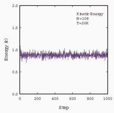
Fig. 3 Kinetic energy of a solid argon system with 108 particles in the simulation cell. The temperature is 20K. The molar volume is 22.3 ml/mol.

 

Fig. 4 Potential energy of solid argon with 108 particles in a simulation cell. The temperature is 20K, and the molar volume is 22.3 ml/mol.

 

Fig. 5 shows the normalized heat current autocorrelation function of a system with 108 argon atoms at temperatures of 10K, 20K, 30K, 40K, 50K, 60K, and 70K, respectively. As temperature increases, the heat current autocorrelation function decays faster. This is due to the fact that there are more scattering processes when the temperature increases.

 

The decay of the heat current autocorrelation function takes place at two stages. A fast decay below 1 ps and a slow decay after 1 ps. The two stages can be seen more clearly in Fig. 6.

 

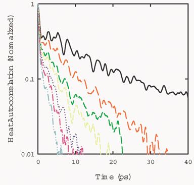
Fig. 5 Heat current autocorrelation function of a system with 108 atoms, at temperatures at 10K, 20K, 30K, 40K, 50K, 60K, and 70K, respectively.

 

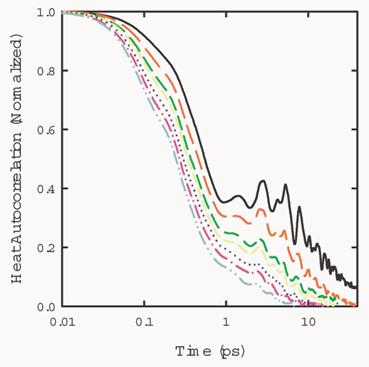
Fig. 6 Heat current autocorrelation function of a system with 108 atoms, at temperatures at 10K, 20K, 30K, 40K, 50K, 60K, and 70K, respectively.

 

Fig. 7 shows the dependence of the thermal conductivity of solid argon on temperature from 10K to 70K. The simulation results are in good agreement with experiment.

 

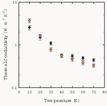
Fig. 7 Thermal conductivity values of solid argon from 10K to 70K. The black circles are experimental values. The red circles are simulation results in a NVT ensemble with 108 particles.

 

Fig. 8 shows the dependence of the thermal conductivity of solid argon on the molor volume at 75K. The results agree with the experimental results.

 

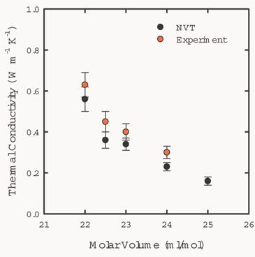
Fig. 8 Volume dependence of the thermal conductivity for a system with 108 particles at 75K in a NVT ensemble.

 

We checked the finite-size effect by repeating the simulations with cubic cells containing of 108, 256, 500, and 864 atoms. Periodic boundary conditions were imposed. The thermal conductivity of solid argon at 50K is converged even with the smallest size considered (N=108), as shown in Fig. 9.

 

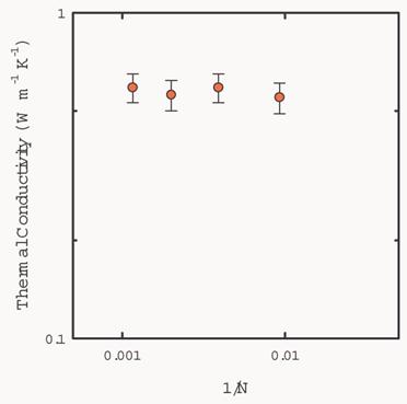
Fig. 9 Calculated thermal conductivity of solid argon as a function of 1/N, where N is the number of particles in the simulation cell. The temperature of simulation is 50K. The molar volume of the system is 22.3 ml/mol.

 

Fig. 10 shows the dependence of the thermal conductivity on the cutoff radius for force calculation in the simulations. The thermal conductivity of solid argon with 108 particles in a cell is independent of the cutoff radius.

 

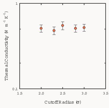
Fig. 10 Calculated thermal conductivity of solid argon as a function of cutoff radius. The number of particles in the simulation cell is 108. The molar volume of the system is 22.3 ml/mol.

 

NPT Ensemble – Methods & Results

Simulation in the NPT ensemble at zero pressure is performed using the constraint algorithm prescribed by Evans and Morriss (1983). Gear’s fourth order predictor-corrector method is used to integrate the equation of motion (Allen & Tildesley, 1987). Temperature and volume are rescaled every 5 MD steps. The integration time step  was set to 0.002  LJ units ~the LJ unit of time is 2.16 ps for argon) at low temperatures (T<50 K) and 0.005  otherwise. The typical lengths of the runs were equal to 1.1x10⁶ MD steps. The LJ pair potential was cut off at a radius of 2.5 and long-range corrections to the energy were considered.

 

The thermal conductivity is calculated by discretizing the Green-Kubo formula:

                 (7)

 

M is the number of steps over which the time average is calculated. M is set to (1-5) x 10⁴ at low temperatures (T<40) and (4-8) x 10³ at higher temperatures.

 

A typical simulation trace of energy and volume after equilibration is shown below:

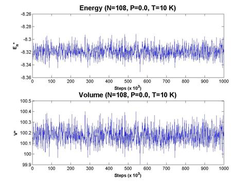
Fig. 11 A typical simulation trace of energy and volume after equilibrium in a NPT ensemble.

 

Next, we present the RMS fluctuations for a typical run after equilibration:

 

Table 1 The RMS fluctuations for a typical run after equilibrium.

N=108, P*=0.0

 

We can see that the system is essentially isothermal and isobaric for the duration of the statistic collection. Fluctuations are on average about 1% of mean.

The normalized heat autocorrelation function are presented below for 7 different temperatures (semilog and linear x-axis). Time is recorded in LJ units (=2.16 ps).

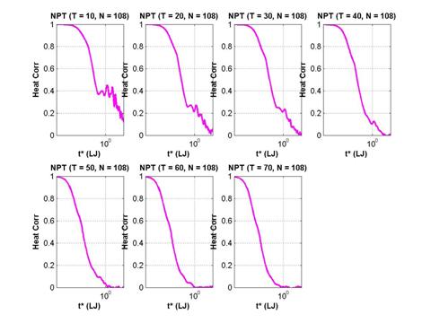
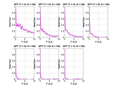
Fig. 12 Normalized heat current autocorrelation function of a solid argon system with 108 particles in the simulation cell.

 

As expected the decay of the autocorrelation function is slower at lower temperature because of the reduced number of scattering events. There is a clear two-stage decay visible – an initial fast component followed by a slower decay. A more detailed analysis of the decay times can be found in Tretiatov (2004).

 

The thermal conductivity obtained is compared to the experimental results. Red markers are from simulation while blue markers are the data of Clayton and Batchelder (1973). We can see the excellent agreement between the 2 data sets even for single runs of 108 atoms. Discrepancies from experiment are less than 25% for the range of temperature considered.

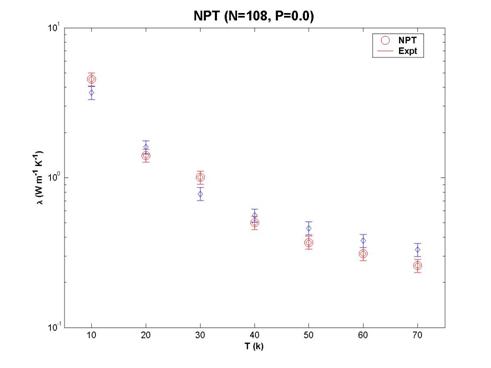
Fig. 13 Thermal conductivity values of solid argon at different temperatures. The red circles are experimental values and the blue squares are the simulation results from a NPT ensemble.

 

To investigate the effect of system size, lattice size from 3-7 unit cells (108-1372 atoms) are simulated at T=50 K. We report minimal finite size effects as demonstrated by the figure below.

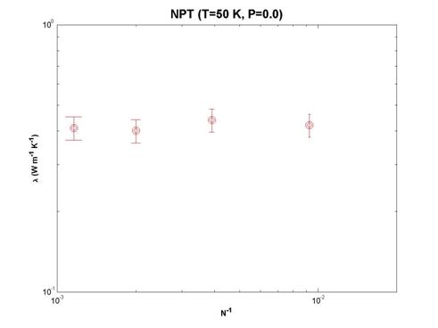
Fig. 14 Calculated thermal conductivity values of solid argon in a NPT ensemble with different number of particles in the simulation cell.

 

Summary

 

We compare the thermal conductivity values calculated from the NVT and NPT ensembles with experimental values in Fig. 15. Both calculated results are in 30% of the experimental values. We conclude that Lennard-Jones potential describes the dynamics of solid argon accurately and the Green-Kubo method is an accurate technique for calculating the thermal conductivity of argon.

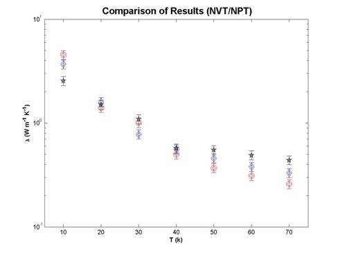
Fig. 15 Comparison of thermal conductivity values obtained from simulations in NVT (black stars), NPT ensemble (blue diamond), and experiment (red circles).

 

References

1. M. P. Allen and D. J. Tildesley, Computer Simulation of Liquids (Clarendon, Oxford, 1987).
2. K. V. Tretiakov et. al. J. Chem. Phys. 120, 3765. (2004)
3. D.J. Evans, G.P. Morriss, Chem Phys. 77, 63 (1983)
4. H. Kaburaki, Ju Li, and S. Yip, Mater. Res. Soc. Symp. Proc. 538, 503(1999).
5. Ph. Jund and R. Jullien, Phys. Rev. B 59, 13707 (1999).
6. F. Clayton and D. N. Batchelder, J. Phys. C 6, 1213 (1973).
7. D. K. Christensen and G. L. Pollack, Phys. Rev. B 12, 3380 (1975).
8. Y. Touloukian, Thermophysical Properties of Matter, Vol. 3, Plenum, New York, 1 (1980).

Source Codes

            Code and Input file for the NVT ensemble.

            Code and input files for the NPT ensemble.

 

Presentation

            Presentation files.