<110> Twist Grain Boundary Energies and Ideal Shear Stress in Pure Nickel
By:
Mike Sangid
Myungeun Suk
May 11th, 2007
Final Project
MSE 485/ Phys 466 / CSE 485
1. Abstract
In this project, the grain boundary
energy is calculated for various twist angles in the <110> direction of
nickel. The reported values are in the
same range as the tilt grain boundary angles found in literature for the same
material and direction [10]. The second
part of the project applies a shear stress on a perfect FCC crystal. The shear modulus calculated is significantly
lower than values found in literature and from experiment. This is a result of a large strain rate being
applied to the crystal in this simulation and the subsequent velocity rescaling
rate in order to keep constant temperature.
In future simulations, the strain rate will be lowered and applied to
twist grain boundaries to find the shear strength of grain boundaries.
2. Introduction
Most metals have a polycrystalline structure comprised of multiple grains, which are bounded by interfacial defects known as grain boundaries. The structure and energetic of these grains gives a microscopic insight for material behavior. One of the most representative examples is the Hall-Petch relationship, which predicts yield strength from the average grain size, although this relationship only deals with the average grain response, thus it is not useful in characterizing the higher ordered effects of grain boundaries such as size distribution and orientation. Grains have a large effect on the mechanical behavior of a material, especially in failure modes such as fatigue, fracture, and creep [1]. Also, grain structures can be quite complicated in real materials, which may contain a distribution of grain sizes with various orientations. Therefore, it can be anticipated that the orientation of these grain boundaries influence the interface properties and as a result the mechanical behavior of the material. Thus, providing the motivation for this study, in which the effects of grain boundary orientation is studied by use of molecular dynamic simulations.
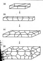
Figure 1. Polycrystalline materials ranging from a bicrystal to a 3D view of a material containing many grains [2].
3. Technical Details
The following sections provide insight and detail concerning the molecular dynamics simulations that were run as part of this project.
3.1 Twist Grain Boundaries in the <110>
Direction
In a FCC material, the preferred slip direction, as a consequence of being the shortest Burger’s vector for dislocations, occurs in the <110> direction [3], hence this represents the most interesting lattice direction for this study. The figure shows a unit screw dislocation with a Burgers vector b=a/2[110] which splits into two Shockley partials. In this figure, the dislocation moves towards the most densely packed (111) plane as a result of a homogeneous ‘out of plane’ simple shear strain.

Figure 2. (a) Schematic of a twist grain boundary [5] (b) A leading edge dislocation in the <110> direction splitting into two Shockley partials [4]
Further, there has been an intensive study of tilt grain boundaries. Thus, this current study of twist grain boundaries (as defined by twisting along the axis shown in the figure above [4]), provides a new outlook to add to the body of work on the subject. Twist grain boundaries are of additional interest, since it provides a unique opportunity to create a coincidental site lattice algorithm. The development of this code offers an insight into the intricacies and complexities of setting up molecular simulations, which is a valuable learning experience.
Nickel was chosen as the material of interest for this study for two reasons. First, nickel is the primary agent used in super-nickel alloys that have many high temperature applications within the aerospace turbine community. Also, nickel has a well established potential, thus making it a good candidate for this study.
3.2 MD Simulation Package – LAMMPS, the EAM
Potential, and Energy Minimization
After, taking some time to compare and contrast the available MD packages that are available, LAMMPS (large-scale atomic/molecular massively parallel simulator) was chosen for a variety of reasons [6]. LAMMPS is an open source code that was developed out of Sandia National Laboratory. The most appealing feature of LAMMPS is that it offers a website containing complete documentation and example input files, thus significantly shortening the learning curve associated with the new package. LAMMPS also offers the Embedded Atom Method (EAM) potential for nickel [7]. EAM is based on density-functional theory, in order to calculate ground state properties of FCC materials. Hence, in this project, the EAM potential is used to model nickel within the LAMMPS MD simulator.
Also, in order to ‘relax’ the lattice structure into it’s preferred atom positions; an energy minimization technique is used known as the conjugate gradient (CG) method. This technique identifies the local configurations that are stable points on the potential energy surface. The conjugate gradient method assumes that the structure is close enough to a local minimum that the potential energy surface is nearly quadratic. Further, all energy minimization simulations are run at a temperature of 0K in this project.
3.3 Perfect
A perfect crystal was constructed in the <110> direction, in order to have a means of comparison, when calculated the energy of a twist grain boundary structure. A unit cell of an FCC structure is shown in Figure 3a [8]. The (110) plane is shown in Figure 3b. Notice that this is a rectangular face with area a√2 by a. Thus, the perfect crystal is constructed by stacking layers perpendicular to the (110) plane, which is also denoted as the <110> direction. Hence, from the schematic, two layers are present, labeled A and B. Each layer has two atoms, although these atoms are distributed differently in the two layers. Layer A has quarter atoms located at the corners and half atoms located in the middle of the top and bottom borders. Layer B has full atoms centered in the plane as shown in Figure 3c. Thus, the rectangles shown in Figure 3c represent a single unit cell, denoted N, and a pair of these rectangles stacked on top of each other in the <110> direction is denoted L. Thus, in the remaining section, lattices are constructed of size NxNxL. For instance, a 2D and 3D view of a 5x5x5 perfect FCC crystal comprised of 1226 atoms is shown in Figure 4.

Figure 3. (a) the FCC unit cell [8] (b) the (110) plane of an FCC cell (c) the stacking layers A-B in the <110> direction (d) the bulk unit cell displaying the size of the given rectangle.

Figure 4. A perfect FCC crystal of size 5x5x5 comprised of 1226 atoms. (a) 2D cross sectional view, which is symmetric in all three directions (b) a 3D view.
3.4 Lattice Constant
The first step in measuring energy through molecular dynamic simulations is to ensure that the correct lattice spacing is used with the associated potential. In order to verify this concern, a plot was generated of the lattice spacing, a, versus the energy of a perfect FCC lattice. As a starting point, the lattice spacing that was determined from experiments (3.5242Å) was used for initial energy calculations; afterwards the energy was taken for small deviations from the experimental lattice constant. A cubic curve fit was created through the plot of lattice energy as a function of the lattice spacing, as shown in Figure 5. From this, the local minimum in energy (the lattice constant where the first derivative of this cubic function is zero) was taken as the simulation lattice constant (3.5240Å). This lattice constant is used in the remaining calculations, as it is the energetically preferred spacing as governed by the EAM potential. Further, the second derivative of this potential with respect to lattice spacing evaluated at the minimum energy results in the bulk modulus of the material. For this fit, the bulk modulus of nickel is 177 GPa, which compares well to literature values of 181-185 GPa. Although, this is of no surprise, since the EAM potential was originally fit to a given material using its elastic constants as fitting parameters [7].

Figure 5. Lattice energy as a function of lattice constant. The corresponding local minimum of this plot occurs at the preferred lattice spacing for this simulation.
4. Twist Grain Boundary Energy
The energy associated with a twist grain boundary in the <110> direction of nickel is calculated in the following sections.
4.1 Energy of a
Perfect FCC Crystal Lattice
Prior to finding the energy of a grain boundary, the potential energy of a perfect crystal needs to be evaluated for means of comparison. A perfect FCC crystal, similar to the one shown in Figure 4, was evaluated using the energy minimization techniques described in Section 3.2. The atoms positions were generated and the LAMMPS code calculated an initial energy of -4.49 eV/atom. The atoms were then allowed to relax and the resulting energy was -4.49 eV/atom. Thus, the atoms were originally in their preferred locations, so the energy did not change. This validates the construction of the perfect crystal and the lattice spacing.
4.2 Coincidental Site Lattice (CSL) Algorithm
In order to invoke periodic boundary conditions, it is necessary to construct a repeating unit cell. Thus, we must find sites where the top and bottom grain both share common ‘in-plane’ positions. These points, known as coincidental sites, can then be used as the corners of the repeating lattice cell [2, 9]. Hence, for certain discrete angles, the two grains in the bicrystal model will have coincidental sites which represent the corners of the periodic repeating lattice. These angles are determined by Pythagorean triplets from the cross-sectional size of the (110) plane in the FCC material. This ensures alignment of the edges of the two crystals thus forming a coincidental site lattice (CSL).
The CSL code that was generated as part of this project is attached. This code allows the user to input the lattice constant (to allow various FCC materials to be modeled in the <110> direction), height of the box, L, and select from a list of appropriate twist angles that result in a CSL. The twist angles then govern the cross-sectional size of the box, N, in accordance with Pythagorean triplets. Thus, the first step in creating this CSL is to create an enlarge lattice, which is referred to as a super-cell. The next step is to create a second lattice of size NxN, which is rotated by the selected twist angle as shown in Figure 6 [9] and ‘stacked’ on top of the super-cell.
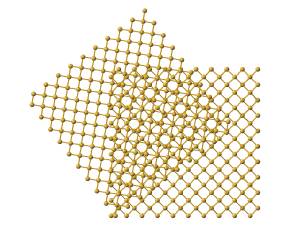

Figure 6. Illustration displaying the top view of a rotation of one lattice with respect to a fixed lattice [9].
Afterwards, additional atoms from the super-cell that do not lie in the same plane (from a top view) as the rotated lattice are removed. Thus, atoms are eliminated from only the base lattice (super-cell) to ensure that both lattices are the same size and share coincidental sites at their corners. Finally, both lattices are rotated back to the corresponding reference frame e1, e2, e3. Thus, one can see the top view and 3D view of a 38.9º and 22.7º twist grain boundary bicrystal in Figures 7 and 8, respectively. Figure 7 is a 5x5x5 unit structure (as previously defined in Section 3.3) with 1,147 atoms, where as Figure 8 has 28,137 atoms in a size of 13x13x20.

Figure 7. A bicrystal with a 38.9º twist grain boundary. This lattice has a 5x5x5 unit structure with 1,147 atoms and was generated using the CSL code.

Figure 8. A bicrystal with a 22.7º twist grain boundary. This lattice has a 13x13x20 unit structure with 28,137 atoms and was generated using the CSL code.
It was pointed out, by the class (which was very much appreciated!), that the bicrystal represented a repeating unit cell. Thus a grain boundary would exist multiple times within each unit cell as the bicrystal was repeated. In order to avoid this, a three lattice - unit structure was created as shown in Figure 9. Thus, the CSL structure would have one rotated grain in the middle of two fixed grains. This results in two grain boundaries per periodic repeating unit.

Figure 9. A CSL structure with one rotated grain sandwiched between two fixed grains representing two twist grain boundaries at an angle of 38.9º. This lattice has a 5x5x5 unit structure with 1,741 atoms and was generated using the CSL code.
The CSL code would then output a file containing xyz coordinates of all the atoms, which is used to create the input file for the LAMMPS program. The code also produced the locations of the corner atoms, which are used to apply boundary conditions. Finally, the code outputted general information to create periodicity, such as the number of atoms and xyz size of the periodic box.
4.3 Periodic Unit Box Size
The next step in the analysis of grain boundary energy is to calculate the size of the periodic box. Thus, the box needs to be sufficiently large to ensure that the grain boundaries do not interact with one another within and across repeating units. Thus, as the box height is increased, the energy per atom reaches an asymptotic value, at which the smallest box size is chosen to increase the efficiency of the code. This procedure is shown in Figure 10 as the lattice structure is relaxed and calculated for a 38.9º twist grain boundary with various box heights, L. For this example, a box height, L=5, is chosen for future calculations of grain boundary energy. It should be noted that this step needs to be repeated for every twist angle.
Figure 10. The box height is determined as the lattice energy is minimized for each box size. The goal is to choose a sufficiently large box height to avoid the grain boundaries from interacting with one another while keeping the overall box size small to increase efficiency.
4.4 Grain Boundary Energy as a Function of Twist
Angle
Once the aforementioned steps are completed, the grain boundary energy can be calculated. The grain boundary energy is calculated from the differences in the total energies associated with the lattice containing the twist grain boundary and the perfect FCC crystal. The perfect crystal (containing M atoms) is normalized to contain the same number of atoms at the twisted crystal (containing N atoms). The grain boundary energy is given as follows:
 (1)
(1)
The ‘unrelaxed’ grain boundary energy is calculated for seven twist angles as shown in Figure 11. The energy minimization algorithm was the run and the grain boundary energy is reported a function of twist angle in Figure 12.
Figure 11. The ‘unrelaxed’ twist grain boundary energy shown as a function of the twist angle for nickel in the <110> direction.
Figure 12. The twist grain boundary energy shown as a function of the twist angle for nickel in the <110> direction.
The values shown in Figure 12 seem reasonable; they vary from 600-1250 mJ*m^-2. Thus, these values are in the same range as tilt grain boundaries in the <110> direction for nickel from a study presented by Seidman [10], as shown in Figure 13a. As Seidman reports, it is expected that this plot has shallow energy cusps. Large grain boundary energies are a product of higher deviations from a perfect crystal configuration. As a result, there is an associated stacking fault with the ordering of the atoms at the grain boundaries. Large grain boundary energies also result in atoms having to climb over one in other to get to their preferred locations. Thus, there exists a large barrier to minimize the total energy of the structure as a result of the twist grain boundary.
Also, twist grain boundaries for a system comprised of silver and nickel is shown in Figure 13b. Again, the values of grain boundary energy fall in the same range as the values presented in this project.

Figure 13. (a) Results for tilt grain boundary energy for nickel in the <110> direction [10]. (b) Results for the energy of (110) twist boundaries in the Ag/Ni system [11].
5. Shear Stress on a Perfect FCC Crystal
5.1. Simulation Set-Up
In this project, a perfect FCC crystal is simulated under shear stress to measure the shear modulus. This method was originally proposed by Horstemeyer [12], in which a shear deformation was applied using the LAMMPS package [6]. Figure 14 and 15 show the snapshot and schematic of the system, respectively.

Figure 14. Schematic of simulation set-up
Figure 15. Snapshot of simulation [12]

![]() Figure
16. Initial velocity field in active atoms
Figure
16. Initial velocity field in active atoms
The crystal orientation for this system is [110, -110, 011] and shear stress was given in <110> direction using boundary condition of constant velocity, as shown in Figure 16. Periodic boundary conditions are applied in the x and y direction. The simulation was performed with a constant number of atoms, constant volume, and constant temperature at 300K (NVT ensemble). The equations of motion were integrated using Velocity-Verlet algorithm with 1fs time step. The Nose-Hoover thermostat [13, 14] and velocity rescaling method [15] was used to keep the temperature constant.
The simulation cell is divided into three regions: lower boundary atoms, active atoms, and upper boundary atoms. The code to sort atoms into three regions and generate the LAMMPS input format is attached. During the initialization of system, the upper boundary and lower boundary atoms were fixed on their perfect lattice sites and active atoms were allowed to relax in order to minimum energy. The initialization was performed for 10,000 steps until the temperature and energy were well maintained, as shown in Figure 17b. Following initialization, strain rate was applied to the upper boundary atoms by setting constant velocity in the x direction and fixing the y and z coordinate of atoms. The lower boundary atoms had zero velocity in the x direction and were fixed on their initial lattice sites.
If the active atoms adjacent to the upper boundary atoms initially experience the given boundary velocity, a shock would be induced into the active atoms due to high strain rates. To resolve this, Horstemeyer et al.[1] introduced an initial velocity field that migrated the shock wave, and then applied boundary velocity fields. An initial x-velocity was varied linearly from 0.0 to the prescribed velocity at the upper boundary atoms according to the z-coordinate, as shown in Figure 16. The temperature was calculated after subtracting this non-thermal velocity initially given. The simulation was run until the active atoms had experienced sufficient strain to create yield. 0.1nm/ps was given as the velocity of upper boundary atoms, and it corresponds to 5.46*10^14 s^-1 of strain rate. Note that strain rate is higher than typical strain rate for simulation, 10^6~10^10, due to the simulation time limitation in our study. This higher strain rate is responsible for deviations from the Horstemeyer paper.

Figure 17. Temperature and energy during initialization
5.2. Results and Analysis
At each atom, the stress tensor can be calculated from:
 (2)
(2)
where i is the atom of interest and j is the neighbor atoms
[2], ![]() is the force vector and
is the force vector and ![]() is a position vector
between atoms i and j, N denotes the number of nearest neighbor atoms, and
is a position vector
between atoms i and j, N denotes the number of nearest neighbor atoms, and ![]() is the atomic volume. To obtain the continuum stress tensor, β
can be averaged over the specimen, i.e.,
is the atomic volume. To obtain the continuum stress tensor, β
can be averaged over the specimen, i.e.,
![]() . (3)
. (3)
Therefore, ![]() was used to plot the
shear stress vs. strain curve in this case. Strain is calculated from the ratio of displacement
to box height, b/a, as shown in the Figure 18.
was used to plot the
shear stress vs. strain curve in this case. Strain is calculated from the ratio of displacement
to box height, b/a, as shown in the Figure 18.


Figure 18. Definition of strain geometry, b/a.
The resulting shear stress and strain curve is plotted in Figure 19. The temperature is maintained by using Nose-Hoover thermostat [13, 14]. Error bars are calculated from the five independent simulations by giving different initial velocity resulting in a Maxwell-Boltzmann velocity distribution. An analysis code to evaluate the stress-strain response is available in the attachment.
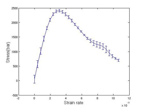

Figure 19. Stress vs. strain curve for <110> perfect crystal
From Figure
19, the maximum shear stress and shear modulus are determined by 0.25 GPa and
0.84 GPa, respectively. Shear modulus is
a hundred times lower than experimental value. Maximum shear stress occurred
within a very short time (0.1ps), and this time was not long enough compared to
the relaxation time of temperature (0.1ps). To remove the heat in a better way during
elastic deformation, velocity rescaling was used with a temperature window 10K.
If the temperature was out of range
(290-310K), then the kinetic energy is rescaled with a factor  every 10 steps. The shear stress vs. strain curve via the
velocity rescaling method is plotted in Figure 20. Each simulation was plotted using a different
color.
every 10 steps. The shear stress vs. strain curve via the
velocity rescaling method is plotted in Figure 20. Each simulation was plotted using a different
color.
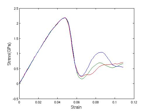

Figure 20. Shear stress vs. strain curve with velocity rescaling
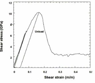
Figure 21. Shear stress vs. strain in <100> direction from [12].
Figure 21 shows Horstemeyer’s work, in which the maximum shear stress and shear modulus were determined to be 2.2GPa and 55 GPa, respectively [12]. The obtained shear modulus is comparable to the experimental value for nickel of 76 GPa. Also, Horstemeyer’s values compare favorably to experiments, since the resulting values for shear modulus are in the same order of magnitude for the <100> direction. It should also be noted, that the material is less stiff in the <110> direction, thus the shear modulus in this direction should be lower than in the <100> direction; although, similar strain rates and velocity rescaling must be used, in order to create a similar means of comparison for these simulations.
6. Conclusions
·
Developed CSL code and generated bicrystal with twist angle grain
boundary.
·
Successfully learned to operate LAMMPS MD code.
·
Determined lattice constants and box dimensions for various twist angles.
·
Calculated the twist grain boundary energy as a function of twist angle
to be in the range of 600-1250 mJ*m^-2, which compared favorably to the results
published in literature for tilt grain boundaries [10].
·
Simulated shear deformation simulation with perfect crystal. The resulting shear modulus (0.84 GPa) was
lower than expected compared to other simulations (55 GPa) [12] or experiments
(76 GPa). This is a result of the
applied shear rate being too high and a low frequency of velocity rescaling.
7. Proposed Work
·
Reproduce the shear stress result with a lower strain rate, in hopes of
increasing the shear modulus.
·
Apply shear stress on a twist grain boundary to simulate the effects of
grain boundary strength with twist angle.
8. References
[1] Suresh S. Fatigue
of Metals.
[2] Phillips R.
[3] Hall D, Bacon DJ. Introduction to Dislocations. BH, Fourth Ed, 2001.
[4] Jin ZH, Gumbsch P, Ma E, Albe K, Lu K, Hahn H, Gleiter H. The interaction mechanism of screw dislocations with coherent twin boundaries in different face-centered cubic metals. Scripta Materialia, 54, 2006, p 1163-1168.
[5] Randle V. The role of the grain boundary plane in cubic polycrytals. Acta Metallurgica, 46, 5, 1997, p 1459-1480.
[6] LAMMPs code documentation. Sandia Research Lab, 2007: http://lammps.sandia.gov/
[7] Foiles SM, Baskes MI, Daw MS. Embedded-atom-method functions for the fcc metals Cu, Ag, Au, Ni, Pd, Pt, and their alloys. Physical Review B, 33, 12, 1986, p 7983-7991.
[8]
[9] Cho B, Reina A, Go D. Constant Temperature Interface Characterization of Silicon Bicrystals. MSE 485 Final Project, 2003.
[10] Rittner JD, Seidman DN. <110> symmetric tilt grain-boundary structures in FCC metals with low stacking-fault energies. Physical Review B, 54, 10, 1996, p 6999-7015.
[11] Allameh SM, Dregia SA, Shewmon PG. Energy of (110) twist boundaries in Ag/Ni and its variation with induced strain. Acta Mater, 44, 6, 1996, p 2309-2316.
[12] Horstemeyer MF, Baskes MI, Plimpton SJ. Computational nanoscale plasticity simulations using embedded atom potentials, Theoretical and Applied Fracture Mechanics, 37, 2001, pg 49-98.
[13] Hoover WG. Canonical dynamics: equilibrium phase space distribution. Phys. Rev. A, 31, 1985, p 1695-1697.
[14] Nose S. A molecular-dynamics for simulations in the canonical ensemble. Mol.Phys, 50, 1984, p 225-268.
[15] Plimpton SJ. Fast Parallel Algorithms for Short-Range Molecular Dynamics. J Comp Phys, 117, 1995, p 1-19.
9. Acknowledgments
We would like to extend our sincere appreciation and gratitude to Prof. Duane Johnson. His tireless and around the clock efforts made this project possible and successful. This project is a result of numerous and lengthy discussions with Prof. Johnson, in which he showed great patience, encouragement, love of teaching, and knowledge, thus giving us the valuable insight needed to complete this project. Further, we would like to thank Dr. Jeongnim Kim and Sandeep Kibey. Dr. Kim took time out of her busy schedule, to explain and help compile an alternative MD code called OHMMS. Sandeep gave us guidance through general discussions about dislocations in FCC materials and their associated stacking fault energy. Finally, we would like to thank the rest of our class for making this an enjoyable experience.
10. Codes
- Coincidental Site Lattice Code (MATLAB code)
- Example <110> Twist Grain Boundary Input to LAMMPS (INPUT txt)
- Shear input file to LAMMPS (Creates Shear INPUT)
- Shear_Stress_Strain_Analysis (Calculates shear output for analysis from LAMMPS)