
Kinetic Monte Carlo Code
The Kinetic Monte Carlo (KMC) technique is attractive for this particluar application due to the fact that there are atomic interactions, which are governed by energy barriers and strongly effect the final state of the system. Furthermore, it is possible to model the system by simply studying the interactions of a single vacancy in the bulk lattice with its nearest and next-nearest neighbors. This quality, which significantly reduces the computation time required, makes the use of other methods that compute forces amongst all particles in the simulation space (i.e. Molecular Dynamics) unattractive, in this case. Furthermore, in this model, an underlying bulk lattice has been assumed over which the atoms are distributed, which makes the KMC technique even more attractive and feasible (1).
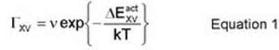
The simulation space is composed of three species: A atoms, B atoms, and one vacancy (V). The A and B atoms can diffuse throughout the simulation space via interaction (or exchange moves) with the vacancy. These interactions are a function of the temperature of the bulk, which makes it possible to construct phase diagrams for the binary alloy from these simulations, though Grand Canonical Ensemble methods are perhaps better suited for this task. The frequency of an A or B atom exchange with the vacancy can be computed via equation 1:(2)
where nu is the attempt frequency, which is derived from kinetic rate theory and is assumed to be unity here. This value does not effect any details of the KMC simulation (it merely scales the relative magnitudes of hopping amplitudes by a uniform factor), but in the calculation of the total simulation time (in physical seconds), it is neccesary. The ball-park value of nu is typically large, (e.g. 1014 Hz), so a rough estimate of the 'physical' time could be obtained by dividing the total number of KMC steps by 1014. Given that a typically run is for 106, 107, 108, or 109 KMC steps, one can assume that the true 'physical' time which is simulated is on the order of 10-8, 10-7, 10-6, or 10-5 'physical' seconds. Even for very long simulations, which might take the better part of a day to run on a fast workstation, only a millionth of a second in real time is being sampled.
The activation energy is then computed via equation 2:
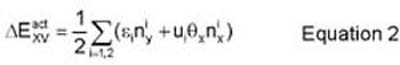
where 'epsilon' and 'u' are (respectively) diagonal and off-diagonal energy parameters chosen in these simulations to fit FeAl (2), 'n_yi' denotes the number of dissimilar atoms in the nearest and next-nearest neighbor shells, 'n_xi' denotes the number of similar atoms in the nearest and next-nearest neighbor shells, and 'theta_i' is an occupancy function which assumes the value -1 for A atoms, +1 for B atoms, and 0 for a vacancy site. This model (and the choice of energy parameters, 'epsilon' and 'u') is described and explored more completely in Athenes (2). For the purposes of this report, the parameter set, (eps1,eps2,u1,u2) = (0.03eV,-0.04eV,-0.04eV,0.0eV), is chosen in accordance with most of the FeAl simulations in Athenes (2), and these values are fixed for all runs. In effect, this energy model is treated as generic and attention is focused on the qualitative features of phases and ageing dynamics.
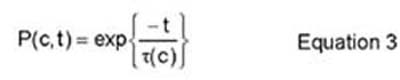
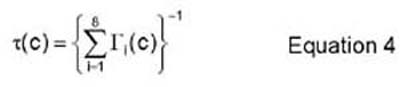
A residence time algorithm is used, in accordance with the model developed by Athenes, et al. The "residence time" eludes to the time that the system resides in a certain configuration. In order for the system to leave its current configuration, the vacancy has to jump to one of the eight nearest-neighbor sites on the lattice. Therefore, after some time, t, the code computes the probability that the system is still in the current configuration. This is done via equations 3 and 4.
where
The action that is taken by the vacancy at each Monte Carlo step is characterized by the number j that satisfies the following inequality (equation 5):
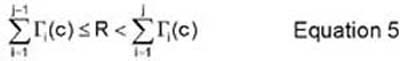
In equation 5, R is a random number that is between 0 and
. This can be more readily viewed as a "probability array", where the array is constructed with the frequencies computed for each move. At a given Monte Carlo step, a random number is generated and the move that the vacancy makes corresponds to where the random number falls on the probability array (the next section discusses how random numbers are generated). It is key to note that as a consequence of the manner with which the probability array is constructed, the vacancy will perform a move at each Monte Carlo step. In other words, it is impossible for a move to be rejected. The probability array is constructed solely of frequencies that correspond to moves to nearest-neighbor sites, so it is physically impossible (in this code) for the vacancy to remain in a given position for consecutive Monte Carlo steps.
Click here to download the KMC code.
Random Number Generator
Two random number generators (RNG) were integrated into the KMC code in order to ensure that the RNG did not affect the results of the simulations. The first generator was adapted from "Numerical Recipes in FORTRAN" and will be referred to as the "Knuth generator", for whom helped develop it.(3) This generator is based on a subtraction algorithm, which is different than most RNGs, making it particularly useful for comparison in the current application. The random numbers are generated on the interval (0,1).
The second random number generator implemented here was adapted from the book "Monte Carlo: Concepts, Algorithms, and Applications" by George S. Fishman and will be referred to as the "Fishman/Moore generator".(4) This is a uniform multiplicative congruential random number generator with modulus 2**31-1. The generator was selected because of the simplicity with which it could be coded and because of the fact that it ensures generation of nonoverlapping pseudorandom number sequences. The random numbers are also generated on the interval (0,1).
Both codes were run stand-alone with three different random seed numbers to prove that the code was generating random sequences. The first generator requires negative seed numbers and the second generator requires positive seed numbers. The mean and error of the mean were computed for a string of 10, 100, 1000, and 10000 numbers generated with the same seed. As is expected for a uniformly distributed number on the interval (0,1), the mean converged to 0.5 and the error of the mean (or the variance) converged to 0.08333, as the number of random numbers generated increased.(5) The time required to generate the longest sequence (i.e. 10000) was much less than a second for both codes, so the generator execution is not the rate limiting step in the KMC code.
One interesting point about the generators can be seen in Figure 1. In the Knuth generator, the variance was small for 10 points (about 0.03) and converged to the expected value of 0.08333, as the number of points increased. In the Fishman/Moore generator, the variance was large for 10 points (about 0.11) and converged to the expected value of 0.08333 as the number of points increased. Intuitively, the behavior in the Fishman/Moore generator is expected, however, the variance for a small number of points should not be important in this study since long intervals of random numbers will be generated.

Figure 1. Left: Knuth generator. Right: Fishman/Moore generator. Proof that the random number generators can generate nonoverlapping sequences from a uniform distribution. All sequences converge to the expected mean and variance for a uniformly distributed number as the sequence gets larger.
The simulations were run with a single random number generator and a single seed, which is usually not done with Monte Carlo codes, since the dependence on the generator and the variance between runs is important to quantify. However, since the main part of the project was the code development, all of the simulations were not run with multiple seed numbers and multiple generators. Several simulations were run with a small simulation cell and multiple seed numbers on both generators. It was found that the variance was not that large in most parameters of interest and the simulations were not dependant on the random number generator used. These results will be shown later.
Click here to download the Knuth RNG stand-alone code.
Click here to download the Fishman/Moore RNG stand-alone code.
Computation of Concentration Field and Degree of Order Field
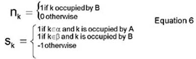
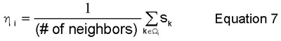
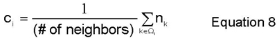
The degree of order field, eta_i, and concentration field, c_i, are computed here by local averaging methods over the set of first and second-nearest neighbor shells, omega_i. In order to perform this local averaging, it is necessary to define variables that quantify what species are where and what structure those species are in. Equation 6 defines two occupancy functions over which eta_i (Equation 7) and c_i (Equation 8) are simply local averages. Thus, at each site, i, in the BCC lattice, these fields return the local average value (over the nearest and second-nearest neighbor shells, omega_i) of the two occupancy functions defined in Equation 6.
It is also helpful to visualize the lattices and sublattices necessary to describe the structure that a certain species is in. The entire bcc lattice that the bulk material is in can be split into two simple cubic sublattices, alpha and beta. These sublattices are required to describe the B2 symmetry, in which the two species segregate with respect to the alpha and beta sublattices. Viewed in the original BCC lattice, the B2 symmetry is seen as a coordination of B-type nearest neighbors about each A atom, and vice versa. These lattices are illustrated below in Figure 2.
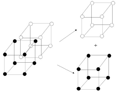
Figure 2. Bulk BCC lattice split into two simple cubic sublattices. The alpha sublattice is on the top right and the beta sublattice is on the bottom right.
Once the bulk BCC lattice is split into the two simple cubic sublattices, the partial order and partial concentration field can be computed for a cell i. These parameters can be computed in the manner depicted in Figure 2. One then plots eta2 for a <110> slice through the bulk BCC lattice to obtain a snapshot of order at a given time. Many of these snapshots can be taken over time and put together to obtain an ageing sequence. One computes eta from equations 6 and 7, which have been written as functions in the code developed here.(2)
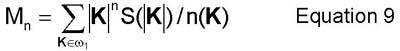
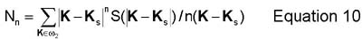
Another method to compute the concentration and degree of order fields is as follows. The structure factor S(K) is the Fourier transform of the pair correlation function g(r). The structure factor is useful in determining information related to the concentration field and the degree of order field. This information is acquired by computing moments of the spherically averaged structure factor S(|K|). Information about the concentration field is gained by computing the moments (Mn) centered around K=0. Information about the the degree of order field can be gained by computing the moments (Nn) centered around Ks. These quantities are defined further in equations 9 and 10.(2)
and
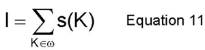
Additionally, the characteristic length of the order field and the characteristic length of the concentration field are computed here as R1 and R2, respectively. These two quantities are computed from the first two moments of equations 9 and 10 (R1=M0/M1 and R2=sqrt(N0/N2)). The integrated intensity of the superlattice reflection is also calculated here by equation 11. From this, S (S=sqrt(I/IB2), where IB2 is the intensity of a perfectly ordered B2 alloy in 1:1 composition), the degree of order can be computed and it can be compared directly to experimental data.(2)
A third method to determine the ordering in the alloy is to compute a long range order parameter (LRO) and a short range order parameter (SRO). The LRO essentially describes the degree of long range order in the alloy by computing the fraction of a certain species in a given sublattice. An example of this would be the number of species A on the alpha sublattice. The LRO is defined such that when the alloy is fully ordered, it equals unity and when it is fully disordered, it equals zero. This LRO is defined below as equation 12. This equation shows that if the alloy composition is not in a 1:1 ratio, then it cannot be fully ordered.(6)
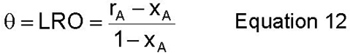
where rA is the fraction of the alpha sublattice occupied by species A and XA is the concentration (fraction) of species A.
The SRO describes the degree of short range order in the alloy. It is different than the LRO because it is computed as a function of the AB bonds in the alloy. The SRO is defined below as equation 13.(6)
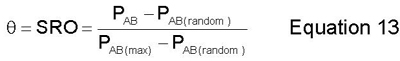
where PAB is the number of AB bonds in the alloy simulation cell, PAB(random) is the number of AB bonds in a random alloy simulation cell, and PAB(max) is the maximum possible number of AB bonds in the alloy simulation cell.
Click here to download the structure factor code.
Results - Phase Diagram
One of the goals of phase simulations here is to show that the code developed here can be used to reflect expected behavior, based on the Iron-Aluminum phase diagram. The theoretical phase diagram can be seen below as Figure 3. Athenes, et al, also cite a similar study where a phase diagram for the Iron-Aluminum system was computed via grand-canonical Monte Carlo simulations. These simulated results can be seen in Figure 4. The phase diagrams are symmetric about 50% concentration, so only one side of the phase diagram is shown.
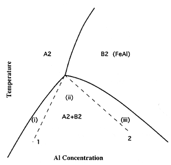
Figure 3. Theoretical Iron-Aluminum Phase Diagram (reproduced from Athenes, et al.)
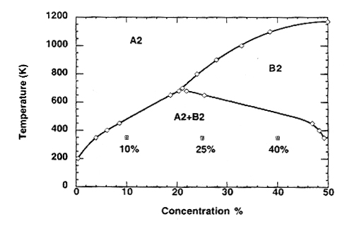
Figure 4. Simulated Iron-Aluminum Phase Diagram (reproduced from Athenes, et al.)
The three phases seen in Figures 3 and 4 can be interpreted as follows. The B2 phase is the ordered phase. When the bulk BCC lattice is split into the alpha and beta sublattices, one species will tend to go to the alpha sublattice and one species will tend to go to the beta sublattice. In this phase, there will be some disorder when the concentration of one of the species is less than 50%, as shown by the LRO. It is key to note that the B2 region on the phase diagram gets larger as the concentration of one of the species approaches 50%. So, the alloy becomes more ordered over a greater temperature range as the ratio of Fe:Al approaches 1:1.
The A2 phase is the disordered phase, or the random phase. From the phase diagrams, it can be seen that, in general, this phase occurs at high temperatures and low concentrations of one of the species.
The A2+B2 phase can be thought of as a combination of the A2 and B2 phase. This phase is actually a two-phase coexistance. In other words, this phase can be thought of as droplets of one phase floating in a sea of the other phase. If one were to look at a slice through an alloy in this phase, it would look like blotches (with some "straglers") of one phase in the other phase. There is not a sharp phase boundary when this phase is present, making it almost an intermediate phase between the A2 and the B2 phases.
Here simulations have been run similar to those performed by Athenes, et al. The temperatures and concentrations were varied and, when viewing the simulation space as two separate sublattices, it is clear that there are very discernable and different phases.
Results - KMC Model Vacancy Path Behavior
In this section, no physical parameters have been calculated. This section is merely intended to show how the vacancy travels throughout the simulation cell.
In Figure A.1 in the Simulations section called "KMC Model Vacancy Path Behavior", the path of the vacancy is plotted during a very small simulation of 256 MC steps in a 16 cell cube. Recall that the vacancy makes a move to one of its nearest neighbor positions at every MC step. It is important to note that in Figure A.1, it appears that the vacancy makes jumps much larger than to one of its nearest neighbor sites. This is just a relic of the plotting package used. When the vacancy is on the edge of the simulation space and it travels to the other side of the simulation space due to the periodic boundary conditions, the plotting package connects the move as a trip across the entire simulation space. Even in this small of a simulation it can be seen that the vacancy traverses a good deal of the simulation space. The simulation was run with the species in a 1:1 ratio.
In Figure A.2, many different alloy compositions were run to determine the effect of alloy composition on the path of the vacancy. Although the results were not very conclusive, the general trend appears to be that as the concentration of the A species in the alloy is increased, the vacancy moves about the bulk material more freely. At lower concentrations of A, the vacancy tends to remain confined to the edges of the simulation space. As the concentration of A is increased, the vacancy appears to travel further in the bulk material. These simulations were also very short and were performed in the same 16 cell cube as in Figure A.1, with 256 MC steps.
Results - Simulations in a 16 Cell Cube
In this section and the following two sections, five simulations were run with varying concentration of species B and temperature. The parameters were selected so that most parts of the phase diagram were sampled (see Table 1). The alpha and beta sublattices were generated for each simulation and can be seen in each corresponding section in the Simulations page. Furthermore, for the 32 and 64 cell cubes, eta2 slices can be seen along with the alpha and beta sublattices. The following are the parameters tested along with the expected phase, as determined from the phase diagram shown previously as Figure 4.
| Concentration of Species B (fraction) | Temperature | Phase |
|---|---|---|
| 0.25 | 700 K | B2 |
| 0.25 | 1000 K | A2 |
| 0.25 | 200 K | A2+B2 |
| 0.05 | 700 K | A2 |
| 0.45 | 700 K | B2 |
Table 1. Points of Interest in the Phase Diagram.
The simulations here were run in a small, 16 cell cube. Each simulation was run for 1*106 MC steps, which was determined to be enough steps to attain the equilibrium structure with this small of a simulation cell. In Figure B.1 of the Simulations section "Simulations in a 16 Cell Cube", it can be seen that there is some definite ordering in each of the sublattices, although the simulation cell is not completely ordered. Complete ordering is not expected, since it can be seen from the phase diagram that this particular combination of parameters is close to a phase boundary.
In Figure B.2 of this same section, a definite random structure exists in both of the sublattices, which is expected for the A2 phase. In Figure B.3, a slightly more ordered structure than in Figure 2 can be seen, although it is not much more ordered than in Figure B.2. This is likely due to the fact that a very small simulation space is used. Therefore, with a small simulation space it is difficult to discern the A2 and A2+B2 phases.
In Figure B.4, a clear random structure can be seen, corresponding to an A2 phase. Finally, in Figure B.5, a highly ordered phase is shown. This is expected, since this concentration of B is close to 0.50. As the 0.50 concentration of B is approached, the structure should become more ordered.
Results - Simulations in a 32 Cell Cube
The simulations here were run in a moderate sized, 32 cell cube. Each simulation was run for 1*107 MC steps and it was determined that this was enough MC steps for the simulations to reach equilibrium. All of the parameters that were run in the previous section were run here and an additional simulation at T=700K and cB=0.50 was run. This additional simulation is at a 1:1 composition and should be in the B2 phase. This simulation should serve as a true check of the model, since there should be a definitive B2 phase present.
In Figure C.1, a clear B2 phase can be seen. This is obvious because there are large clusters of one species in the alpha sublattice and only a limited amount of that same species in the beta sublattice. Additionally, the eta2 plot shows clusters of values of eta2 greater than 0.5 (chosen arbitrarily), meaning that there are large groups of ordered atoms.
In Figures C.2 and C.3, a greater contrast between the A2 and A2+B2 phases can be seen than in the 16 cell cube. In the Figure C.2 alpha sublattice, the red species is much more randomly distributed throughout the cell than in the Figure C.3 alpha sublattice. There is much more clustering of the red atoms in the alpha and beta sublattice in Figure C.3, though not as much as in Figure C.1, which is characteristic of the A2+B2 phase. The eta2 plots in Figures C.2 and C.3 are relatively indistinguishable, which leads to the conclusion that this method of determining phases is not highly reliable.
Figures C.4, C.5, and C.6 illustrate a sharp contrast between the A2 and B2 phases. In Figure C.4, there is no ordering at all and this is reflected in the eta2 plot, where no values were greater than the 0.5 cutoff. In contrast, there is a high degree of ordering in Figures C.5 and C.6. In Figure C.6, there is almost complete ordering, which can be seen in the alpha and beta sublattices. This claim of a high degree of ordering is also substantiated by the eta2 plots.
Results - Simulations in a 64 Cell Cube
The simulations here were run in a large, 64 cell cube. Each simulation was run for 1*107 MC steps, which turned out to be likely not enough steps to resolve the equlibrium structure for each pair of parameters. A possible explanation for this is that since the simulation cell is larger than in the previous set of simulations (with the same number of MC steps), the vacancy does not have enough time to explore the full simulation cell.
In Figure D.1, there is some obvious ordering, which can be seen in the alpha and beta sublattice and the eta2 plot. The alpha and beta sublattices in Figures D.2 and D.3 are virtually indistinguishable. Additionally, the eta2 plots indicate that the simulation in Figure D.2 is more ordered than Figure D.3, which is not likely, since Figure D.3 is the more ordered phase. This is one indication that these are not equilibrium structures.
Figure D.4 is very similar to the analagous plot for the 32 cell cube. There is clearly no ordering in either sublattice and the eta2 plot is empty, as it was for the 32 cell cube. In contrast, there is clear ordering in Figure D.5. However, the degree of ordering is not as high as in the analagous smaller cells. This is another indication that this is not an equilibrium structure.
Results - Order Parameter Output
The results of all of the order parameter computations can be seen in the Order Parameter Output section. In Figure E.1, the ideal B2 structure has been generated and is shown. Then, in Figure E.2., the corresponding long range and short range order parameters are shown. These two figures serve to show the expected behavior, both visually and numerically, of the B2 phase.
In this section the RNGs were tested by computing various quantities with three different seeds in the two RNGs previously described. It is shown here in Table 2 that the mean and the variance in all of the quantities do not vary significantly between the RNGs, meaning that it should not matter which RNG is used to perform simulations with this code. Furthermore, the variance in most of the quantities is relatively small, so the approximation of running one simulation to show phase behavior is not a terrible approximation. In a future study with this code, one would compute running averages of each of the quantities in Table 2 and determine where the averages converge. The convergence point would dictate how many simulations would have to be run with different seed numbers in order to guarantee that one is reporting the true mean and variance that would be obtained for a given parameter with this code.
Knuth's Subtractive RNG1 Fishman/Moore Linear Congruential RNG2 Order Parameters Mean Variance Mean Variance LRO 0.082 0.020 0.075 0.031 SRO 0.9059 0.0049 0.9095 0.0019 R1 0.03309 0.00026 0.033855 0.000086 R2 1.749 0.028 1.8126 0.0056 I1 (FCC) 2.7619 0.0093 2.763 0.014 I2 (SC) 2.626 0.056 2.630 0.057 Table 2. Results of Order Parameter Calculations for Three Seed Numbers on Two Random Number Generators. FCC=Face Centered Cubic. SC=Simple Cubic.
The following plots in this section are order parameter results of simulations shown in the Ageing Seuqnces section. As shown in Figure E.3., the long range order parameter (LRO) basically increases with ageing time and reaches its saturation value of 0.2 after about 7 intervals (or 7*108 MC steps). However, the curve does not increase monotonically. The fluctuations in the curve are due to a large variance in the LRO parameter, as shown in Table 2. It is important to note that here a very small system (16 cell cubic) is simulated, which contributes to the large varience in the LRO parameter.
The short range order parameter (SRO) is shown in Figure E.4. The SRO parameter increases to a high level very quickly in the first 6 intervals (or 6*108 MC steps, and then continues to increase slowly with ageing time.
The results shown in Figures E.5 and E.6 can be compared to the work by Athenes, et al.(2) In Figure E.5 R1 is plotted versus MC step and does not compare to the analagous curve computed by Athenes. However, the curve shown in Figure E.6 does compare well to the analagous curve by Athenes. On explanation for this strange behavior is that the simulation cell here is very small compared to that used by Athenes, so a true concentration and order field might not be sampled here. Finally, in Figure E.7, it is shown that when B atoms form an ordered B2 structure with A atoms, the excess A atoms will form a BCC structure on the simulation lattice. Therefore, the diffraction intensity from the ordered B2 structure and BCC structure will increase during the ordering process. The reciprocal lattices for the two set of simple cubic sublattices in B2 are still simple cubic. The reciprocal lattice for BCC is FCC. By calculating the diffraction intensity from these two reciprocal lattices one can monitor the structure change in ordering. Therefore, the diffraction intensity from the simple cubic reciprocal lattice and the FCC reciprocal lattice are shown in Figure E.7.
Results - Ageing Sequences
In this section, a high temperature quench was performed and the results were visualized. Order parameter data for these simulations were shown in the previous section. In Figure F.1, an ageing sequence is shown as plots of eta slices with an arbitrary cutoff of 0.7. The simulation was quenched from 700K to 348K at 8*107 MC steps. The simulation is a total of 5*108 MC steps. The temperatures were selected in accordance with Athenes.(2) In Figure F.2, a similar simulation was performed. This time more MC steps were performed and the visualization method is different. The quench from 700K to 348K was done at 4*108 MC steps, with a total simulation time of 2.5*109 MC steps. The blue dots are either species A or B and the white dots are the ordered B2 domain.
It proved to be difficult to distinguish the growth mechanism that was occuring here in Figures F.1. and F.2. The two possible growth modes were proposed to be the continuous mode and the nucleation and subsequent groth mode. The ageing sequences that were created helped to discern what mode was occuring, however, the simulations appeared to equilibrate faster than expected, making it difficult to observe the phase transition behavior from the disordered to ordered phase. It is believed that the nucleation and growth mode is occuring, which is suggested from observations of the first couple of frames of Figure F.2. Small "blotches" of the ordered phase appear and quickly expand. There does not appear to be a time continuity in the transition.
Conclusions
This KMC code has proven to be viable in generating expected equilibrium phase behavior, based on the phase diagrams presented for this system in Athenes, et. al. Given a certain temperature and alloy composition, the code will generate the correct equilibrium phase, provided that enough MC steps are taken for the given lattice size. This is true because as the lattice size increases, the number of MC steps to reach the equilibrium structure increases. One area that was not addressed here was distinguishing phase transitions. This could be done by searching for kinks in the free energy diagram, critical slowing down, or finte-size-scaling phenomena. It would be possible to perform a study such as this with the code developed here, but it was not done for this project since a large amount of time was devoted to code development.
In addition to verifying the existence of three phase regimes, dynamical growth and ageing was observed, as visualized by mapping the magnitude of the degree of ordering field over planes of the lattice. Nucleation and growth mechanisms were confirmed, and the time of transit from a disordered distribution to a two-phase coexistence state was estimated.
A further study with this code would involve varying the energy, u1, to determine the energy effects on the simulations that were run for this study. This was done by Athenes, et al, where they observed the vacancy behavior at various energies. It would also be instructive to calculate the total free energy, in order to observe phase transitions and the order of discontinuity in moving across phase boundaries.
References
(1) Hybrid Monte Carlo method for off-lattice simulation of processes involving steps with widely varying rates. Clark, M.M., Raff, L.M., and Scott, H.L. Computers in Physics, Vol. 10, No. 6, Nov/Dec 1996.
(2) A Monte-Carlo Study of B2 Ordering and Precipitation Via Vacancy Mechanism in B.C.C. Lattices. Athenes, M., Bellon, P., Martin, G., and Haider, F. Acta Metallurgica. Vol. 44, No. 12, pp. 4739-4748, 1996. (and additional personal communication with Bellon)
(3) Numerical Recipes in FORTRAN: The Art of Scientific Computing. Second Edition. William H. Press, Saul A. Teukolsky, William T. Vetterling, and Brian P. Flannary. Cambridge University Press. New York. 1992.
(4) Monte Carlo: Concepts, Algorithms, and Applications. Fishman, George S. Springer-Verlag New York, Inc. New York. 1996.
(5) Probability and Statistics for Engineers. Fourth Edition. Richard L. Schaeffer and James V. McClave. Duxbury Press. Belmont, California. 1995.
(6) Elements of X-Ray Diffraction. Cullity, Bernard D. Addison-Wesley, 1978
Here are some relevant web references:
Atomic Scale Simulations in B2 NiAl