Melting on the Surface of a Sphere
by Dongxiang Liao and Robert Furstenberg, part of a
course project for MatSE
390AS
Introduction
In this project we studied the entropy-driven phase transition of
a system of hard-disks on the surface of a sphere.
We chose this topic mostly because we didn't find any code or
literature dealing with constant NpT simulation on a spherical
surface. We would like to see how the implementation and results
differ from other approaches.
The goals of our project are as follows:
- Write a complete Monte Carlo program for simulating the two
dimensional hard disk system, implementing the constant pressure constraint and spherical boundary condition;
- Obtain the equation of state for the
system and radial distribution functions
(RDF) at different density;
- Compare the results with those by other methods.
Theory
Entrop driven phase transition of hard disks
Allen and Tildesley[1987] gave an excellent
review of simulation of melting in their book Computer
Simulation of Liquids. The tutorial paper by Gould et al.[1997] is very helpful for beginners.
Here, we would just give a brief introduction of the background of our
study. Interested surfer should consult the book and the reference
therein.
The pair potential u(r) between hard disks is given by
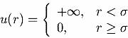
where the r is the distance between the disks and s is the diameter of the disks. We notice that
the interaction is purely repulsive, so there is no distinct gas and
liquid phases. The disordered phase is generally referred to as a
fluid.
The existence of fluid-solid transition for hard disks at
sufficient high density was one of the first major discoveries from a
computer simulation. Alder and Wainwright[1962]
did a molecular dynamics simulation of a 870 hard-disk system with
periodic boundary condition. They concluded that the hard-disk
melting is first order. The also found that melting density is 0.691
and the freezing density is 0.716 (Here we express the density in
terms of packing fraction which gives the ratio of the area of the
disks to the container area). However, since a phase transition exists
only in the thermodynamic limit, it would not be possible to simulate
the fluid at the critical point with small systems and finite time.
The results could depend strongly on the system size and the nature of
the hard-disk transition is still a evolving problem.
"Spherical boundary condition"
Computer simulations are usually performed on limited small number
of molecules. Periodic boundary conditions (PBC) are the standard
method for eliminating the surfaces. Periodic boundary will be biased
in favor of the formation of a solid with a lattice structure which
matches the boundaries. Most PBC studies of hard disks use a box
ratio of sqrt(3)/2, which favors the formation of single perfect
hexagonal lattice. As a result, the equation of state depends on the
system size, with larger system encouraging higher transition
pressure. Possibly reason is that more defects or even an hexatic
phase is allowed to exist in sufficiently large systems[Zollweg and Chester, 1992]
The surface of a sphere has no physical boundaries, yet it is
finite. This neatly avoid the surface problem. According to
non-Euclidean geometry, the distance between particles is measured
along the great circle geodesics joining them. However, the curvature
effect will decrease as the system size grows, and such method should
be valid for simulating bulk fluid. The advantage here is that there
is no preferential direction and it is impossible to pack particles
into a perfect close packed configuration.
Constant-NpT Monte Carlo
Wood [1968] first showed that MC method can be
extended to isothermal-isobaric ensemble. We use constant-NpT method
due to the following consideration:
- In constant-NpT ensemble, The pressure is set as a input
parameter, the calculation of the equation of state is more
direct. Specifically, the pressure need not to be calculated by
extrapolation of radial distribution function to the contact value.
- At constant N, P, T we should not see two phases coexisting in
the same simulation cell, as in canonical ensemble.
The Metropolis scheme is implemented by generating a Markov chain
of states which has a limiting distribution proportional to

where s = r/Radius is a set a scaled coordinates. A
new state is generated by displacing a disk randomly or making a
random volume change from Am to An. Moves are
accepted with a probability equal to 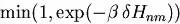 , where

Programming details
We select the particles to move sequentially. After one sweep (one
attempted move per particle), an attempt to change the volume is
made. In practice, we change the lnV instead, which is more convinient
for the case volume change is large. The only change to the
acceptance/rejection procedure is that the factor N is replaced by
N+1. In the hard disk case, a particle move is rejected if it cause
overlap, accepted otherwise; the volume decrease is accepted if no
overlap happens; the volume increase is accepted with probability  .
.
Programs are written in FORTRAN 90. You can find the source code
here.
Example of an input file
100                     ! run_id
0                       0/1 - use existing configuration/generate new
946374734               random seed
100.0                   betaP
0.1                     max_move_ratio (max_move/sigma)
0.002                   max_dlnA (about max_resize/area0)
10000                   # of blocks
10                      # sweeps in each block
The initial configuration can be read in or generated randomly. In
the first case, a "config.dat" file is needed; in the latter
case, the shortest distance between particles is chosen as the disk
diameter. The initial radius of the sphere is 1.0. The max random
move size is usually chosen so that the acceptance ratio is close to
0.5. After a successful run, following files are generated.
run_id.log
- record the initial condition and the final status
run_id.cfg
- the final configuration
run_id.sca
- record the change of density
/scratch/run_id.crd
- record the configurations at certain interval (big file)
Analyzer
is used to analyze the density data. The mean is obtained by
averaging data from 100,000 -- 200,000 sweeps, depending on the the
length of autocorrelation (typically nubmer is 1700 for a 120-disk
system at density 0.61). The long correlation time pose a challenge
for the psuedo random number generator. In our calculations, the
intrinsic generator of the Sun UltraSPARK 2 machine is used. We
believe that better random number generator is necessary for
simulation of larger systems.
Program rdf.f90 is then used to
calculate the radial distribution function from
run_id.crd. Generally, a segment of 500
configuration is used.
Results
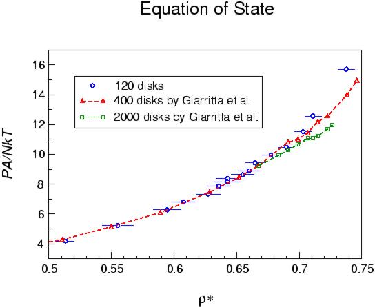
Equation of state
The equation of state is obtained by calculating the densities at
different reduced pressures (P/kT). Figure 1
shows the results of our 120 hard disks system compared with
constant-NVT simulations of larger systems[Giarritta et al., 1992]. The agreement is very well
up to the density of 0.67. The discrepancy at higher pressures is
most likely due to size effect, as explained by Giarritta. With a 2000
disk system and more extensive calculation of the isothermal
compressibility(numerical differentiation of the EOS curve), they
concluded that
- at density lower than 0.67, the system is a fluid and without
ordering, it is insensitive to curvature effect;
- density 0.67 to 0.71 is a regime that the system undergo the
transition from fluid to solid;
- at higher density, the change is a continuous one towards
higher spatial ordering.
Our results generally support their conclusion. However, the
exact density at which the transitions happen is not clear from our
plot. We did not see a certain pressure range that the variance of
the density is very large. This is possibly due to the very long
correlation time of the simulation or the phase transition is not
abrupt.
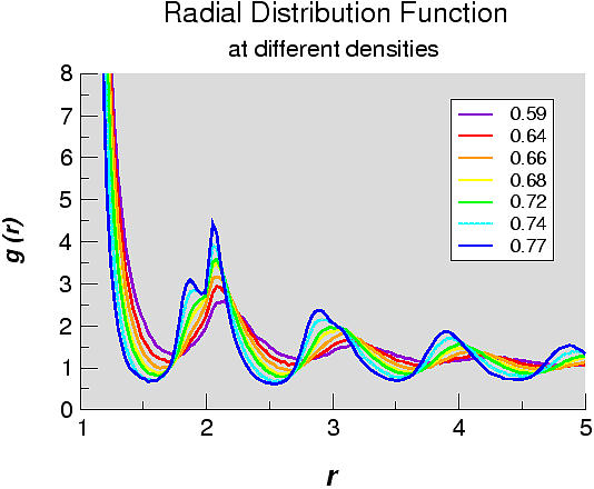
Radial distribution functions
Figure 2 shows the RDF of 120 hard disks for a
number of densities in the range of interest. The radial distance is
plotted in the unit of the disk diameter. Although RDF is not very
sensitive to local structures than orientational correlation
functions, it is easily calculated and can be used to visualize the
phase transition approximately. We can the see a split second peak
typically of an amorphous solid or glass breaks out at a density of
about 0.72. This value is close to 0.71 obtained by Giarritta et al.
Summary
- It is effective to use constant-NpT ensemble to study this
phase transition. The direct information about pressure is
especially convenient;
- The fluid-solid phase transition on a sphere shows continuous
characters. Generally, the results depend on the the system size.
Method to scale the result on the sphere need to be developed;
- Alder, B. J. and Wainwright, T. E. (1962). Phase transition in
elastic disks, Phys. Rev. 127, 359-61.
- Allen, M. P. and Tildesley D. J. (1987). Computer
Simulation of Liquids, Oxford University Press, Oxford.
- Giarritta, S. P., Ferrario, M. and Giaquinta, P. V. (1992)
Statistical geometry of hard particles on a sphere,
Physica A 187, 456-74.
- Gould, H., Tobochnik, J. and Colonna-Romano, L. (1997).
Computer in Physics, 11, 157-163.
- Tobochinik, J. and Chapin, P. M. (1988).
J. Chem. Phys. 88, 5824-30.
- Wood, W. W. (1968). Monte Carlo calculations for hard disks in the
isothermal-isobaric ensemble, J. Chem. Phys. 48,
415-34
- Zollogand, J. A. and Chester, Melting in two dimensions,
G. V. (1992). Phys. Rev. B. 46, 11186-9.
d-liao@uiuc.edu
Dongxiang Liao
Department of Materials Science and Engineering
University of Illinois
Urbana, IL 61801