For an active walker system, by changing the range of scaping function,
which is essentially the range of interaction, and
then calculating the fractal dimension of the resulting pattern, we
had the following dependence.

We can see the fractal dimension decreases as R(Range) increases.
Let N be the number of occupied sites.
We can derive a semiempirical formula for the fractal dimension.
For a square, A = r2. So dA = 2rdr. On a lattice, r = k
(k = 0,1,2,...)
dr = dk = 1. So dA(k) = 2k.

dA(k+1) = ((k+1)/k)*dA(k) = dA(k)*(1+1/k). (1)
From this iteration fromula we can get,
dA(k) = (k/(k-1))*((k-1)/(k-2))*...*dA(0) = Const*k ~ k1.
A square obviously has dimension 2. So the exponent in this formula is dim-1.
We will develop a formula similar to (1) to calculate the fractal dimension.
Assume in a given pattern, dA(k) = n(k) at kth layer(k-1 -- k), since
no walkers
die until they hit the boundary. All the n(k) walkers will go to the
next
layer(k -- k+1). Aside from these n(k) walkers, there are also 1/k
extra unocupied
sites for each walker in average. The reason is because we use squares
with
increasing side length to cover the pattern to calculate the fractal
dimension.
From (1), (dA(k+1)-dA(k))/dA(k) = 1/k. Whether the 1/k sites will be
occupied or not depends on the scaping function. Let R be the Range
of scaping
function specified in the program. When R is large, the sites besides
a occupied
one will be depeleted more, so the probability those sites will be
the next one
the walker goes to is less.

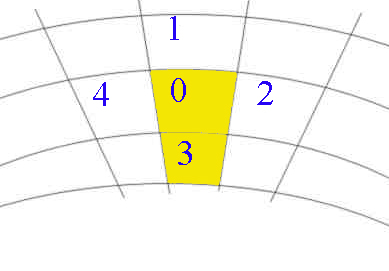
The current walker is at site 0. Site 3 is occupied. There are 3 choices
left.
The probability of walking to a site depends on how much 1, 2 and 4
is depleted,
which depends on how the occupied sites distribute around them.
Site 2 and 4 are surrounded by more sites than site 1 since site 1 is farther
away from those occupied sites.
If R = 1, no lanscape is modified, the value at each site is always
1, so site 2 and 4 will be eventually occupied.
If R is very large, the landscape value at site 2 and 4 is much less
than site 1
since there are more occupied nearer to site 2 and 4 to deplete its
scape value.
Site 2 and 4 then can hardly be occupied.
At a very crude approximation, we can let probability to site 1, P(1),
= cR.
c is a constant to be determined. So P(2 or 4) = 1-cR. To get a better
fit
to the data, we use instead P(2,4) = 1+d - cR, with d is
a small number
acting as a correction.
So now we have,
dA(k+1) = n(k+1) = n(k) + n(k)*(1/k)*P(2,4)
= n(k) + n(k)*(1/k)(1+d-cR)
= n(k)(1+(1+d-cR)/k)
(2)
Note 1+d-cR = p(2,4) < 1. So its higher power goes to zero. We can
rewrite (2) as
n(k+1) ~ n(k)(1+(1+d-cR)/k+((1+d-cR)(1+d-cR-1)/2)*k2+...)
(finite series)
= n(k)(1+1/k)1+d-cR
So n(k+1) ~ ((k+1)/k)1+d-cR * (k/(k-1))1+d-cR
*... n(0)
= (k+1)1+d-cR n(0)
We can see that
Dim ~ 1+1+d-cR = 2+d-cR.
Using this formula, do a linear least square fit to the data, we can
get.
d = .03(Small!), c = .05.
Dim = 2.03-.05*R.
The graph is as following.
It can reflect the approximate relation of fractal dimension
with R.
We can also see relation 2+d-cR2is a better formula.