To investigate the effects of a grain boundary in a binary alloy, a Monte Carlo (MC) simulation was run using two different codes, CLAMPS and, EAM. The two codes, differ only in the way the potential energy is computed. As was discussed in the theory section, for metallic solids, the binary LJ interaction does not give accurate values for potential energy. EAM is a method, that has been widely used for describing metallic systems. In effect, we would like to see how, these two methods compare in simulating grain boundary segragation.
CLAMPS code was obtained from Dr. Ceperley. Original EAM code was obtained from Dr. Folies. In the two codes we used the same MC algorithm for chosing and moving the atoms. To more efficiently explore the phase space, an additional type of step was added to CLAMPS algorithm. In the EAM code, the existing implementation was made more efficient by choosing the atoms to be of different type in the scheme described below.
In the standard Metropolis Algorithm, only random movements of atoms are computed. However, in a solid it may take many steps for atoms in neighboring lattice sites to interchange. Instead of randomly moving one atom at a time, it is more efficient to interchange the type of two randomly choosen atoms. The acceptance probability for this Monte Carlo step is computed using the difference in the potential energy between the unswapped and swapped configurations.
It is important to note that in this algorithm atom types are interchanged instead of positions. This is computationaly more effective, because this operation do not change the neighbor lists.
Now as the atoms are swapped they create a strain on the lattice. In the CLAMPS code, the lattice was relaxed during the simulation by performing standard Metropolis steps (moves) with a small box size (0.08). The ratio of swaps to moves was set at 5. For a given step, the step type was randomly chosen with moves having probability 0.2, thus giving the desired ratio.
The method of relaxation was somewhat different in the EAM code, which is though to achieve the same goal of removing the strain created by type interchanges. The exact method is as follows:
In the CLAMPS simulations, the starting lattice was read in from a previously created file. This initial configuration ([001] twist grain boundary) was created as follows. First the program Creator was used to create a perfect fcc lattice of a large dimension. A typical dimension was 14x14x20 in number of unit cells on a side. Solvent atoms were then replaced at random by solute atoms until the desired concentration was obtained. After converting to the CLAMPS lattice format, the initial lattice was reflected across the x-y plane at one end of the z-direction, with the resulting lattice being shifted to be centered on the origin. Next, for the portion of the lattice with positive z-coordinates a given rotation was applied about the z-axis. To prevent the problem of having atoms on the edge of the box, the x and y coordinates were then shifted by 1/4 of the lattice constant. Finally, all atoms outside of the desired lattice box were deleted. Thus a lattice was created with a twist boundary in the x-y plane at z=0 (and also in the x-y plane at the z-periodic boundaries).
After running the simulations, the concentration as a function of distance in the final lattice was computed. This was accomplished by computing the number density of the specified atom in bins along each coordinate axis. The size of the bins was taken to be the lattice constant for the system.
| Atom Type | Lattice Const (A) | Cohesive Energy (eV) | Sigma (A) | Epsilon (eV) |
| Pt | 3.92 | 5.84 | 2.54 | .679 |
| Au | 4.08 | 3.81 | 2.65 | .443 |
The simulations were run in dimensionless units obtained by normalizing the value of sigma to that of Pt, and epsilon to that of Au. This gives Pt a sigma of 1 and Au a sigma of 1.04. As well, Pt has an epsilon equal to 1.53 and Au has epsilon equal 1.
It remains to fix the cross interaction parameters. It is reasonable to set the sigma of the interaction to the average of the sigmas of the two components, as sigma represents the approximate "hard" radius. This gives sigma equal to 1.02. In determining epsilon, we must make sure that for our desired composition and temperatures of interest that the binary alloy is in the 1-phase region. That it does not phase separate. To accomplish this task, a perfect Pt fcc lattice was created with 8 unit cells in each dimension. The lattice was then randomly populated with Au atoms until the desired composition was obtained. For various values for the epsilon of interaction MC steps of both types were run for over 200000 iterations. By examining the concentration profile of the resultant lattice every 50000 steps, one may determine whether the system is phase separating. If so, then local concentration of the Au atoms will much larger than the average. The system can also be compared to the initial state to see how it has evolved.
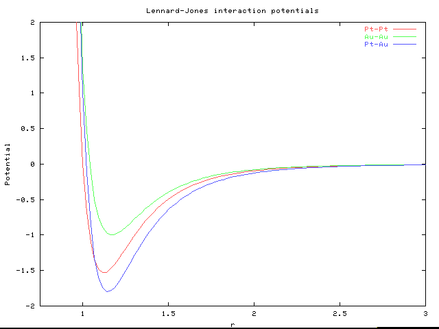
The four temperatures 10K,100K,300K,and 800K were run with epsilon varying between 1.0 and 1.8. It was determined that for this range of temperatures, an epsilon of 1.8 would provide the best alloy properties. This value, larger than the two self-interaction epsilons, seems reasonable as the different types of atoms must be more strongly attracted to the other than to its own type of atom. The final potential are show below.

Following are some example concentration profiles. A bin denotes an average over a unit cell in the given direction.
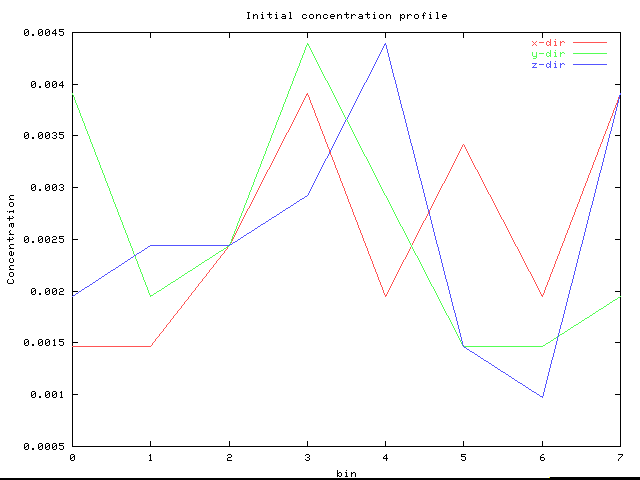
This random profile sets the range of fluctuation which will be acceptable after many MC steps. Note that the average value for the concentration is .0025.
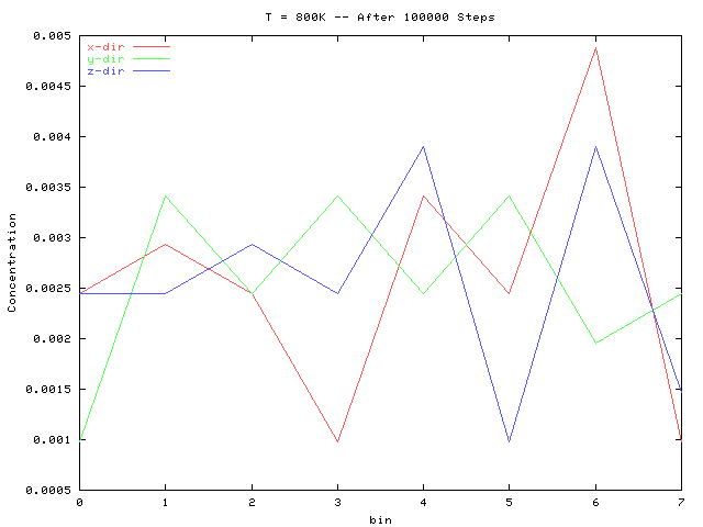
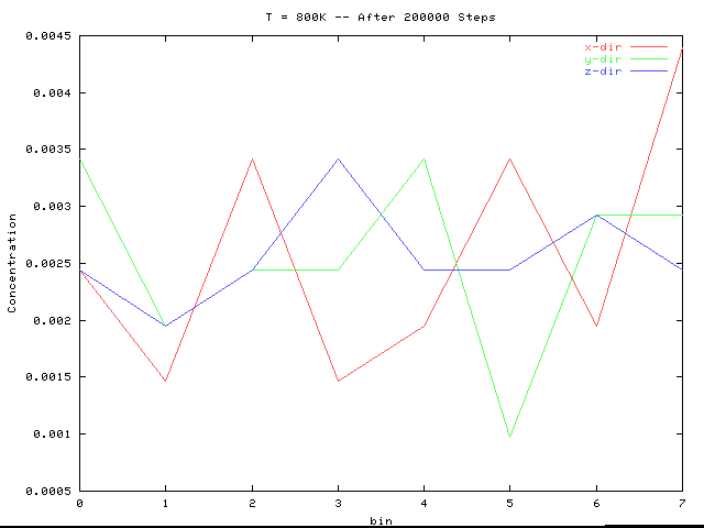
The above two plots are for an interaction epsilon of 1.8. Note that their concentration fluctuations lie within that of the initial lattice, and no longer contains a large correlation at bins 3 and 4 as did the initial configuration.

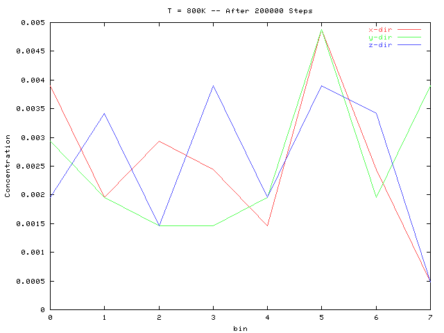
The above two plots are for an interaction epsilon of 1.0. It is clear
that for the large time (bottom plot) the system is undergoing phase separation
at bin 5, where the concentration in each direction is much greater than
the average. Similar results to these were seen at the other temperatures
examined.