Constant Temperature Interface Characterization
of Silicon Bicrystals
Ben Cho, Alfonso Reina, Daniel Go
MATSE 385 Final Project Report
PowerPoint | Movie1 | Movie2 | Movie3
1. Bicrystals and interface between flat surfaces
The
theoretical investigation of bicrystal behavior is extremely relevant to a
wide range of matrerials phenomena, such as grain boundary interfaces in metals,
and atomic friction recently observed by AFM techniques. There has been much
effort implemented to understand the relations between a material’s
microstructure and properties. Study of the simplified situation of a single
grain boundary interface can give insight into the much more complicated phenomena
underlying microstructural dynamics. Therefore there has been a simplification
of systems of interest as depicted in fig.1 [1]. The discussions and simulations
contained in this project refer to the case illustrated in fig 1a. This configuration
represents a preliminary investigation of the more complex case referring
to polycrystals.
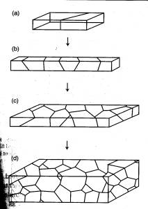
Figure 1:
Different kinds of polycrystals
At
the micron scale level inside a material, there are multiple grains that comprise
a typical crystalline solid as illustrated in figure 1d. These different regions
are bounded by interfaces known as grain boundaries. For a bicrystal, this
interface is the region uniting two differently oriented lattices of the same
material. Therefore, the study of these characteristic regions of bicrystal
systems provides insight into the nature of grain boundaries.
In addition, friction is responsible for a wide range
of important phenomena in scientific research despite a paucity of knowledge
about the atomistic causes underlying its behavior. Atomic friction is currently
a topic of great scientific interest due to its impact in AFM microscopy and
nanoscience. The work undertaken by Gyalog et al. is a good example of the
issues being addressed [2]. For instance, the friction between extended atomically
smooth surfaces is relevant to investigate phenomena occurring in currently
performed nanosled experiments, where defined islands of C60 are dragged over
a NaCl substrate. Varying results for the interfacial friction behavior observed
between two atomically flat surfaces have been obtained for different models.
Figure 2 illustrates the interfacial friction dependence on the sliding direction
between two surfaces of materials. The authors of this research paper simulated
particles classically by assigning specific spring constants to them. In addition,
fig.3 shows data relating friction force per particle as function of the misfit
angle between the two slabs of material [2]. It can be seen that there are
well-defined angle-dependent maxima and minima of the frictional force value.
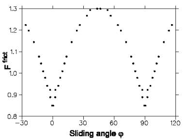
Figure 2: Friction force for different sliding directions
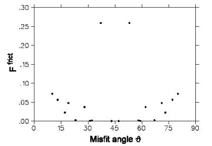
Figure 3:
Friction force for different misfit angles.
The
project here presented has been limited to the case of silicon bicrystals
generated by rotating two parallel slabs with respect to each other and with
along the (001) zone axis as depicted in fig. 4. Nose-Hoover thermostat control
has been implemented for constant temperature simulation. Additionally, lateral
translations were added to the rotated configuration of the two slabs in order
to analyze the position-dependent energetic behavior of the resulting system.
2. Objectives
·
Generate a silicon bicrystal by rotating two silicon slabs with respect to
one another.
· Implement a Nose-Hoover thermostat control to employ constant temperature
simulations of the aforementioned silicon slabs.
· Study the energetics and structure of the bulk system and interface for
a specific rotational angle as a function of lateral translation and temperature.
3. Computer Simulations
3.1 OHMMS
OHMMS
(Object-Oriented High-Performance Multi-Scale Materials Simulator) is a C++
based program created by Dr. Jeongnim Kim. Under her guidance, we implemented
a Nose-Hoover thermostat control to the OHMMS code. The items that were added
to her program are:
·
A modification to an already existing Leapfrog integrator in OHMMS to include
the Nose-Hoover thermostat.
· An algorithm to generate the atomic positions of two silicon slabs rotated
with respect to one another, given angle of rotation, lateral translation,
slab separation, and system size.
3.2 Preparation of bicrystal sample
To
simulate twist bonded interfaces one starts with two perfect supercells and
rotate one with respect to the other by a certain angle. To ensure periodic
boundary conditions for both crystal parts, we need an enlarged supercell.
For certain angular rotations lattice points of the bottom lattice will coincide
with lattice points of the upper lattice. This is known as a coincident site
lattice [1 ].
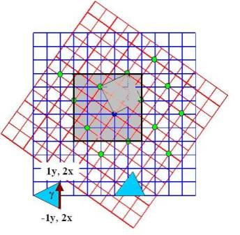
Figure 4:
Coincident lattice for rotated simple cubic 2D slabs
Therefore, for certain angles, there is a periodicity cell that defines the
particular points at which both lattices coincide. We expect important differences
in the behavior between cases with different periodicity cell of their coincidence
sites, e.g. different “magic” angles. Angles that give this coincidence
condition are of the form [2]:
cos  =
a / N cos = b / N a, b, and N are
integers
=
a / N cos = b / N a, b, and N are
integers
The
integers a, b and N comprise a Pythagorean triplet. Every Pythagorean triplet
can be generated from two integers p and q (p > q) by a=p2 – q2,
b=2pq, N= p2 + q2, and the permitted angles are given by:
tan /2 = q/p
Fig. 5 illustrates the geometrical significance of a, b and N inside the pattern
formed by the two rotated slabs with lattice constant equal to one for simplicity
[2]. The number of special angles that can work for a specific system strongly
depends in the size of the lattices. Therefore, if a specific angle which
corresponds to a specific triplet, there is a minimum size the slabs should
have. Pythagorean triplets are presented with their respective angle of rotation
in table 1 shown below.
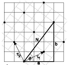
Figure 5:
Schematic illustration of a, b and N and the corresponding vectors
t1 and t2 of the smallest common periodicity cell in a coincidence
site lattice.
| a |
b |
N |
|
| 1 |
0
|
1 |
90 |
| 3 |
4 |
5 |
36.8698 |
| 5 |
12 |
13 |
22.6198 |
| 7 |
24 |
25 |
16.2602 |
| 9 |
40 |
41 |
12.6803 |
| 11 |
60 |
61 |
10.3888 |
| 13 |
84 |
85 |
8.7974 |
| 15 |
112 |
113 |
7.6281 |
| 17 |
144 |
145 |
6.7329 |
| 19 |
180 |
181 |
6.0255 |
Table 1: Examples of pythagorean
triplets with their respective rotation angles
Table
1 is only a partial listing of the many Pythagorean triplets possible. When
implementing the coincidence site lattice theory to a silicon lattice composed
from a unit cell like the one shown in fig 6, the coincidence angles are the
same as the ones calculated in the previous table due to the square geometry
of the silicon unit cell (see fig. 5). The only difference is that the lattice
constant is not 1 but 5.43 Angstroms for the three directions, which permit
us to use the same angles calculated for the Pythagorean triplets.
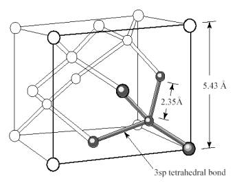
Figure 6: Silicon unit cell
When
rotating two parallel silicon slabs as described previously, it is possible
to obtain the vectors that span the coincidence site lattice (CSL) or smallest
periodicity cell represented in fig. 5 by the green points. These are shown
below:
 1
= N½( e1 cos j/2 + e2 sin
/2 )
1
= N½( e1 cos j/2 + e2 sin
/2 )
2
= N½( -e1 sin j/2 + e2
cos /2 )
In
order to include all the atoms that are contained in this coincidence site
lattice and to simplify the algorithm to reproduce the twisted bicrystal structure
for the simulation, the grayed-out section of fig. 4 was chosen to be the
base supercell. This was then expanded periodically to generate a sample of
the bicrystal with specific dimensions depending on the desired sample geometry.
Due to the complexity and time required to run Molecular Dynamics and Nose-Hoover
algorithm, this project has been limited to the specific rotation angle of
36.8698º, which corresponds to the (3,4,5) Pythagorean triplet. To generate
the coordinates of our rotated supercell, we first created an expanded version
of the base supercell and applied rotation to the coordinates using the relationships
[2]:
Xnew = X cos
- Ysin
Y new = X sin + Ycos
The
expanded lattice was used to account for the area left unoccupied over the
original unit cell as a result of the rotation, as illustrated in figure 7a.
Using the expanded supercell, and applying rotation, and discarding points
that fall outside of our original cell boundaries, we obtain a slab structure
as shown in figure 7b.
(a) (b)
Figure 7:
(a) Illustration showing effect of rotation only.
(b) Illustration of final slab structure
3.3 Nose-Hoover Thermostat, Leap Frog integrator and code implementation
Molecular
Dynamics simulations have typically been done with a constant energy ensemble
or microcanonical distribution. This is somewhat inappropriate when considering
that the majority of experiments in the laboratory are made at constant energy
conditions rather than constant overall energy of the studied system. Nose
proposed a way to accomplish constant temperature simulations by the introduction
of an extended Hamiltonian of the system, which had an additional term Q corresponding
to an artificial mass interacting with the system. Later, Hoover modified
this Hamiltonian and its respective equations of motion and so the Nose-Hoover
dynamics were obtained. The Nose-Hoover extended energy is described by :
And
this results in the Nose-Hoover equations of motion:
3.4 Potentials
3.4.1 Stillinger-Weber Potential
The
Stillinger-Weber Potential is one of the first attempts to simulate silicon
with a classical model. The potential is based on a two-body and three-body
term. It is built to favor four-fold coordination bonding between atoms just
as seen in the silicon structure.
This potential gives a very good description of crystalline silicon but doesn’t
work well for conditions different from those it was designed for. Therefore,
it does not give accurate information of surface structures and energies,
due to the fact that surface atoms have coordination different for that of
bulk atoms.
3.4.2 Tight Binding Potential
In
Tight-Binding schemes for silicon each atom is associated with a finite set
of orbitals, or atomic basis states, each of which can be occupied by two
electrons. To describe bonding in silicon requires a minimal (s,p) basis consisting
of one s orbital and a set of three rotationally related p orbitals for each
atom. Four bonding electrons are distributed among these orbitals. Occupation
of the s and p orbitals by an electron requires on-site energies Es and Ep,
respectively. The coupling of the orbitals of nearby atoms promotes bonding.
The
disadvantage of Tight Binding is that it is a more computationally intensive
due to the fact that it considers multi-atom interactions over a relatively
long length scale, which requires a significant increase in computing power.
Note:
Due to the interfacial surfaces to be studied through this project, Tight
Binding potential was chosen as a first option for the simulations presented.
Later on, Stillinger-Weber was used due to the unavailability of computational
resources necessary to compute a 400 atoms Tight-Binding simulation necessary
for our generated rotated slabs. It is expected that the results obtained
with Stillinger-Weber are not technically correct. However, it is possible
to investigate energetic behavior of the silicon slabs using Stillinger-Weber
to find characteristic behavior of the interface for different configurations.
Due to the short range nature of the Stillinger-Weber potential, the distance
between slabs was made relatively small in order to ensure interaction between
surface atoms of the two slabs.
3.5 Temperature controlled simulations for 36.8698 degree rotation and
different translations.
The
first step following generation of the lattice positions of the rotated lattice
was to determine the lateral translation of this rotated lattice that would
result in a lowest energy configuration.
Ten possible lattice translations were investigated, 5 along each of 2 possible
translation angles, 0º and 45º, in increments of L/10 and (L*20.5)/10 where
L=5.43 angstrom (bulk Si lattice constant as shown in fig.8.
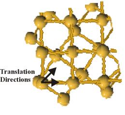
Figure 8. Vectors for initial lattice translations
Next,
to find which of these lattice configurations corresponded to the lowest energy
state, the following procedure was performed:
·
At 0K, steepest descent algorithm from OHMMS was implemented to promote the
relaxation of the system at 0 ºK. This way, it was possible to relax the system
and allow it to rearrange into a low-energy configuration characteristic of
the lattice translation applied.
· The system was heated up to a temperature of 1000 ºK using the leapfrog-Nose-Hoover
algorithm in OHMMS . Entire system and interface energies were recorded at
the end of the simulation.
· Finally, the sample was cooled down to 0K using steepest descent algorithm
from OHMMS. Once again, entire system and interface energies were recorded.
· The final configuration energies (interfacial and entire system) were compared
to find which one of the ten translations gave the lowest (most stable) arrangement
of the interface atoms.
· The configuration found at the previous point was used to simulate different
constant energy behavior of the silicon bicrystal at: 200, 400, 800, 1000,
1200, 1400, 1600, 2000, and 3000 ºK.
4. Results
To
implement correctly the developed Nose-Hoover thermostat, it was necessary
to find an appropriate value for the artificial mass of the algorithm. The
criteria used to determine it was that the correct value should give a minimum
standard deviation or minimum in temperature fluctuations, the nearest value
of the temperature mean to the temperature pursued and of course a Gaussian
distribution of the temperature values for the particular MD run. In a Nose-Hoover
simulation, the energy that is conserved is not the system under study but
the entire system including the Nose artificial mass. To analyze the reliability
of the thermostat code programmed, energy conservation was recorded for some
MD runs of the twisted silicon slabs. Fig. 9a shows the temperature trace
obtained for one of the attempts to implement the Nose thermostat code presented
in Bond’s paper in one of the twisted slab systems. It is evident that
the overall energy keeps increasing with a constant slope. The problem was
that the equation of motion of the friction factor had the term gkT, which
made the equation size dependent due to the multiplication between g and T.
Thus, a minor modification of the Nose-Hoover implementation presented in
Bond’s paper was required, consisting of dividing by g, thus normalizing
the quantity as seen in the equations of motions shown previously. After fixing
the problem and repeating the simulation, energy conservation was accomplished.
This is illustrated in Fig. 9b.
Figure 9a: System energy calculated using incorrect Nose-Hoover thermostat
Figure 9b: System energy calculated using correct Nose-Hoover thermostat
Figure 10: Thermostat-controlled system temperature (1000 ºK)
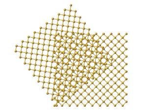
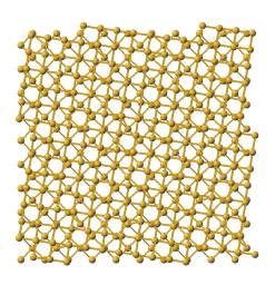
A schematic of the atomic positions for the translation resulting in the lowest
energy configuration is shown in figure 11a. It may be seen that in this initial
state there is relatively little bonding in the interface, thus this is a
quite unrealistic configuration. Performing a steepest descent calculation
on this arrangement results in the configuration shown in figure 11b. The
formation of a significant number of tetrahedral bonds is evident.
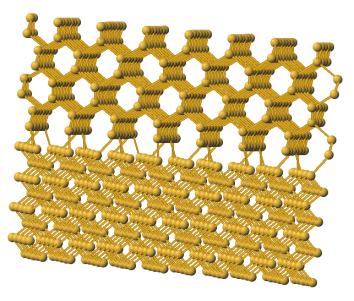
Figure 11a: Initial system configuration
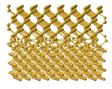
Figure 11a: System configuration after 1st steepest descent calculation
After determining the most suitable value for the artificial mass in the Nose-Hoover
thermostat for the twisted silicon slab system, the MD simulations were performed
as described in the previous section. Figures 12a and 12b show the results
obtained for the (a) total and (b) interface energies of the system as a function
of lateral translation of the upper rotated slab. Well defined minima can
clearly be identified, which correspond to stable configurations of the twisted
slab system.
Figure 12a:
Total system energy results for different lateral translations
Fig. 12b: Surface energy results for different translations
Atomic images from the constant temperature MD runs for the lateral translation
of the rotated slab leading to minimum system energy are shown in figures
13a, b, c, and d for temperatures of 200, 600, 1200 and 2000 ºK.
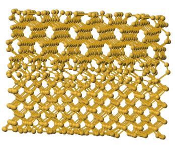
Fig. 13a
Constant temperature configuration at 200 K
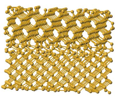
Fig. 13b Constant temperature configuration at 600 K
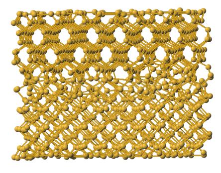
Fig. 13c Constant temperature configuration at 1200 K
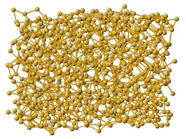
Fig. 13d Constant temperature configuration at 2000 K
It can clearly be seen that the lattice becomes more disordered as the temperature
of the system is increased, and that past the melting point all long-range
order in the system is lost. Unfortunately, from simple visual examination,
the manner in which the character of bonding at the interface changes with
temperature is not immediately apparent.
The interface energy as a function of temperature is plotted in figure 14.
Additionally on this graph, interface energy for low and high energy translations
is shown for T = 1000 ºK. The interface energy exhibits a rising trend with
temperature. The difference in surface energy for high and low energy translations
was 0.000497. No clear difference in interfacial structure is visually apparent
for these two structures, as shown in figure 15 a (low) and b (high).
Fig. 14:
Interface energy as a function of temperature
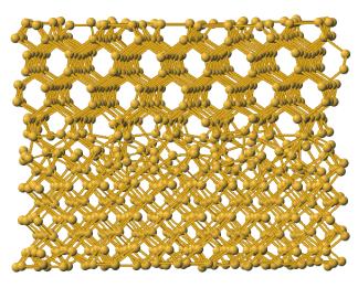
Figure 15a: Interface configuration
obtained for a low energy lateral translation
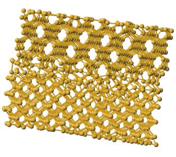
Figure 15b: Interface configuration obtained for a high energy lateral
translation
Finally,
the total system energy as a function of temperature is shown in Figure 16.
The onset of melting is apparent as a large jump in the system energy near
the theoretical melting temperature of Si (1687 ºK).
Fig. 16:
Constant temperature configuration at 2000 K
5. Conclusions
To
restate our experimental objectives, we set out to:
·
Generate a silicon bicrystal by rotating two silicon slabs with respect to
each other.
· Apply a Nose-Hoover thermostat control to implement constant temperature
simulations.
· Study the energetics and structure of a specific low energy rotational case
as a function of temperature and lateral translation.
With
respect to the first point, it was possible to implement Coincidence Lattice
Site theory to find a smallest common periodicity cell when rotating two silicon
slabs with respect of each other. Therefore, periodic boundary conditions
were developed correctly by the usage of this method to fabricate the twisted
slab system. Although we focused the results to only one case of rotation,
there are many other combinations of rotation angle and supercell dimension
that can be implemented.
Referring
to the second point, Nose-Hoover thermostat was successfully implemented,
correctly maintaining a constant temperature ensemble along with a verlet-based
leapfrog propagator. The criteria used to find a suitable Q mass value was
that for that specific value, it was imperative to have a minimum in the standard
deviation of the temperature trace, a maximum proximity to the temperature
desired and a Gaussian distribution of these temperature values through the
MD run. Also, another indicator of the correct functionality of this thermostat
is the conservation of the total energy (slabs system plus Nose Q mass system
or heat bath) as shown in figure 9b.
We
found a clear dependence of the system and interfacial energy on lattice translation,
with well defined minima corresponding to low-energy atomic configurations.
The interfacial energy of the slabs increased with increasing temperature,
while the difference in interfacial energy between high and low energy translations
seemed to be minimal at best, with a value of
EHIGH-ELOW = 0.000497. Below the melting temperature we found the system energy
to be constant with increasing temperature. Once the temperature reached >1600
ºK we observed a large jump in the system energy corresponding to melting
of the slabs.
6. Future Investigations
There
are a number of areas where this study can be continued. First is the quantitative
statistical analysis of interfacial bonding and structure as a function of
temperature, lateral translation, and slab separation. Also, this study can
be extended to other rotation angles. Ideally a generic lattice expansion
algorithm could be implemented to allow automatic calculation of coincidence
site geometry and supercell size. Finally simulation employing alternate potentials
such as MEAM or tight-binding can provide more a accurate simulation of atomistic
behavior and serve as a valuable complement to the information obtained in
this study.
7. Appendix
Nose-Leapfrog
algorithm code snippet
//////////////////////////////////////////////////////////////////
// (c) Copyright 2003- by Jeongnim Kim, Benjamin Cho, Daniel Go, Alfonso Reina
//////////////////////////////////////////////////////////////////
//////////////////////////////////////////////////////////////////
// Jeongnim Kim
// National Center for Supercomputing Applications &
// Materials Computation Center
// University of Illinois, Urbana-Champaign
// Urbana, IL 61801
// e-mail: jnkim@ncsa.uiuc.edu
// Tel: 217-244-6319 (NCSA) 217-333-3324 (MCC)
//
// Supported by
// National Center for Supercomputing Applications, UIUC
// Materials Computation Center, UIUC
// Department of Physics, Ohio State University
// Ohio Supercomputer Center
//
//////////////////////////////////////////////////////////////////
// -*- C++ -*-
#include "Propagators/NoseLeapFrog.h"
#include "Potentials/PotentialBase.h"
#include "ParticleBase/ParticleUtility.h"
using namespace OHMMS;
NoseLeapFrog::NoseLeapFrog():
ToApplyBConds(false), T_ref(0.0), Dt(1.0), Chi(0.0)
{
nose_ke_ind = E.add("Nose-KE");
nose_pe_ind = E.add("Nose-PE");
addParameter(T_ref,"temperature","K");
addParameter(Dt,"timestep","fsec");
addParameter(Q,"Q","fsec-1");
addParameter(Chi,"Chi","nose-var1");
addParameter(Theta,"Theta","nose-var2");
}
bool
NoseLeapFrog::propagate(PotentialBase* pot) {
ParticlePos_t& F = *myPtcl->getVectorAttrib(FORCE_TAG);
ParticlePos_t& V = *myPtcl->getVectorAttrib(VELOCITY_TAG);
ParticleScalar_t& Eloc = *myPtcl->getScalarAttrib(ENERGY_TAG);
ParticlePos_t& R0 = *myPtcl->getVectorAttrib(TRAJECTORY_TAG);
Tensor_t stress;
// ************* degrees of freedom *************
Scalar_t g = static_cast<Scalar_t>(OHMMS_DIM*myPtcl->getTotalNum()-1);
if(!Initialized) {
reset(false,false);
pot->set(myPtcl); // assign a particle set to PotentialBase::myPtcl
Initialized = true;
F = 0.0e0;
Eloc = 0.0e0;
E[PotEnergy] = pot->evalForce(F, Eloc, stress, 0);
evalAccel(F);
}
// ************ Eval velocity at t+dt/2 *************
Scalar_t v0 = 1.0/(1.0+Chi*Dtover2);
Scalar_t v1 = Dtover2/(1.0+Chi*Dtover2);
V = v0*V+v1*F;
// ************* Eval position at t+dt *************
R0 += Dt*V;
// ************* Eval Theta at t+dt/2 *************
Theta += Dtover2*Chi;
// ************* Eval Chi at t+dt *************
evalKineticEnergy();
Chi += DtoverQ*(2*E[KineticEnergy]-g*KE_ref);
// ************* Eval Theta at t+dt *************
Theta += Dtover2*Chi;
// ************* Update the force with R0 at t+dt *************
myPtcl->updateR(R0);
F = 0;
Eloc = 0;
stress = 0;
E[PotEnergy] = pot->evalForce(F, Eloc, stress, 0);
evalAccel(F);
// ************* Eval velocity at t+dt *************
v0 = 1.0/(1.0+Chi*Dtover2);
v1 = Dtover2/(1.0+Chi*Dtover2);
V = v0*V+v1*F;
// ************* Eval Kinetic Energy at t+dt *************
evalKineticEnergy();
// ************* Eval Nose-KE
and Nose-PE *************
E[nose_ke_ind] = Chi*Chi*Q*0.5;
E[nose_pe_ind] = g*KE_ref*Theta;
// ************* Eval total
energy *************
E[FreeEnergy] = E[PotEnergy] + E[KineticEnergy] + E[nose_ke_ind] + E[nose_pe_ind];
Counter++; // increment
the internal counter
bool moving = (E[Temperature] > zeroKelvin);
E[Now] += Dt;
return moving;
}
void NoseLeapFrog::reset(bool trescale, bool wrapping)
{
resetBase();
// reset, time coefficients with new or old MD parameters
Counter = -1;
Dtover2 = Dt/2.0;
DtoverQ = Dt/Q;
if(!Initialized) {
KE_ref = Kelvin_to_eV*T_ref;
//Q *= amu_to_mass_unit;
ParticlePos_t& V = *myPtcl->getVectorAttrib(VELOCITY_TAG);
ParticlePos_t& R0 = *myPtcl->getVectorAttrib(TRAJECTORY_TAG);
///////////////////////////////////
// these values are always in cartesian coordinates
///////////////////////////////////
R0.InUnit = false;
///only R0 has to be added to the position data to
which boundary conditions apply
myPtcl->addPositionAttrib(R0);
//if(fabs(E[Now]) < zeroKelvin && T_ref
> zeroKelvin) {
if(fabs(E[Now]) < zeroKelvin) {
///needs to assign Velocity, if not initialized
if(T_ref>zeroKelvin && E[Temperature]<zeroKelvin) {
setVelocity(T_ref);
}
}
convert(myPtcl->Lattice, myPtcl->R, R0);
}
// scale temperature with the new parameters
if(trescale) setTemperature(trescale,T_ref);
if(Initialized && wrapping) myPtcl->applyBConds();
}
...
8. Acknowledgement
We would like to give our thanks
to many people whose guidance and suggestions are critical in making our simulation
project possible. Many thanks go to Dr. Jeongnim Kim of Materials Computation
Center for her generosity in time and effort on helping us debugging the Nose-Hoover
thermostat in her OHMMS program, and suggesting the topic as well as the practical
issues on the simulation. Many thanks go to Professor Stephen Bond of the
Department of Computer Science at UIUC, for his published work on simplified
implementation of Nose-Hoover algorithm. His private discussion with one member
of the group is appreciated. Many thanks go to Professor Kurt Scheerschmidt
at Max Planck Institute of Microstructure Physics of Halle, Germany, for his
invaluable suggestions on the use of Pythagorean triplets and Coincidence
Site Lattice theory for determining the correct misfit angles. Finally, many
thanks go to Professor Johnson for his general discussion, excitement, patience
and encouragement on his students' projects.
9 . References
1) Phillips, Rob. Crystals, Defects and Microstructures. Cambridge University
Press
April 2000. United Kingdom
2) Gyalog, Tibor et al. Atomic Friction. Zeitschrift
Fur Physik B.
3) Foll, Helmul. Defects in Crystals.
University of Kiel.
http://www.tf.uni-kiel.de/matwis/amat/def_en/index.html
4) Bond, Stephen et al.
The Nose-Poincare Method for Constant
Temperature
Molecular Dynamics. Journal of computational Physics 151(1999)114-134