A Comparative Study of GROMACS and NAMD

Yanbin Wu, Joonho Lee, Yi Wang

Team Project for Phys466

May 11, 2007

Abstract:

We compare two molecular dynamics (MD) packages GROMACS and NAMD for different water models and temperature control schemes. A periodic system of water with and without ions were investigated and a total of 20ns simulatioins were performed. The two MD packages were found to produce similar results using the same set of parameters. The damping coefficient in langevin dynamics temperature control scheme was found to affect the dynamics of the system dramatically.

Introduction

Water constitutes about 70% of the human body. Because of its physiological significance in the metabolism of all living organisms, water is the most commonly used solvent in both biological experiments and computer simulations involving biomolecules. Thanks to its simple structure and homogeneous nature, water is an ideal system for comparing different simulation programs and benchmark important parameters, e.g., temperature control parameters, used in MD simulations.

The two MD programs GROMACS (Lindahl et al., 2001) and NAMD (Phillips et al., 2005) are both widely used MD simulation packages with somewhat different emphasis: while GROMACS aims at fast simulations, NAMD is targeted at parallel computing of large systems. Many aspects of an MD simulation can cause different results using the two MD packages. For instance, the force fields used by the program are usually different. Other causes include long range potential calculation algorithm, e.g., PME or Ewards for electric interaction, basic simulation parameters such as time step, neighbor list cut-off radius, as well as temperature control scheme like Langevin, Berendsen or Nose-Hoover method. Usually SPC/E rigid water model (Berendsen et al., 1987) is utilized with Nose-Hoover or Berendsen temperature control scheme in GROMACS, while flexible TIP3P (Mahoney and Jorgensen, 2000) water model is commonly used with Langevin control scheme in NAMD.

Here we compare the two packages using a periodic system of water with and without ions. During our comparisons, we tried different combinations of all controllable parameters in the two packages. For details please refer to the appendix I. Our results indicate that using a same set of parameters, the two packages yield very similar results. Two different water models, SPCE and TIP3P were compared and it was found that the two models appear to have similar dynamic properties. We have also found that the damping coefficient in langevin dynamics may affect the simulation results dramatically and therefore has to be chosen with caution.

Below we describe the procedure of our simulations first, and then we present the results as well as analysis obtained from these simulations.

Methods and Results

Locate a zero point

Before any comparison of the two packages, we tried to first locate a ``zero point'', which allows us to evaluate the results produced by the two programs using the same set of parameters. A microcanonical ensemble (NVE) was used in which no temperature and pressure control are applied. The water box, 30Å in all dimensions and consisting of 2685 atoms (see appendix), was simulated for 1 ns using both GROMACS and NAMD. The fluctuation in total energy, temperature and radial distribution function were compared, as shown in Fig.1 to 4. Diffusion coefficients were also calculated and compared as a dynamic property of the system, as listed in Table 1.

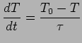
It is noteworthy that the force fields used by MD programs are often optimized at 300K. Therefore, in order to simulate our NVE ensemble at this temperature, a short (250 picosecond) ``warm-up'' simulation was performed to bring the system's temperature up to 300K. In order to eliminate any interference from the different temperature control schemes used by the two programs, this warm-up simulation was only carried out with NAMD. The final coordinates and velocities of the system was retrieved and used as a starting point for the microcanonical ensemble simulation.

After the NVE simulation, a NVT ``zero point'' was also acquired using a similar procedure. Langevin dynamics was used in both GROMACS and NAMD in these simulations. The result for the NVT zero point simulations are shown in Table 2. According to the NVE and NVT simulations, diffusion coefficients calculated using the two packages are only 5.6% and 7.3% for NVE and NVT, respectively.

Compare temperature control schemes

Berendsen, Nose-Hoover and Langevin dynamics are all commonly used temperature control schemes in MD simulations (Frenkel and Smit). The berendsen thermostat mimics weak coupling with first-order kinetics to an external heat bath with a given temperature. A deviation of the system temperature from T$_0$ is slowly corrected according to

$$\frac{dT}{dt}=\frac{T_0 - T}{\tau}$$

in which the temperature deviation decays exponentially with a time constant $\tau$.

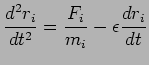
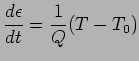
The Nose-Hoover algorithm extends the system's Hamiltonian by introducing a thermal reservoir and a friction term in the equations of motion. The friction force is proportional to the product of each particle's velocity and a friction parameter:

$$\frac{d^2r_i}{dt^2}=\frac{F_i}{m_i} - \epsilon \frac{dr_i}{dt}$$

$$\frac{d\epsilon}{dt}=\frac{1}{Q}(T-T_0)$$

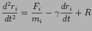
Compared with Nose-Hoover method, Langevin Dynamics introduces a random force, the equation of motion becomes:

$$\frac{d^2r_i}{dt^2}=\frac{F_i}{m_i} - \gamma \frac{dr_i}{dt}+R$$

$$\langle R_i(t)R_j(t+s) \rangle = 2m_i\gamma k_b T \delta(s)\delta(ij)$$

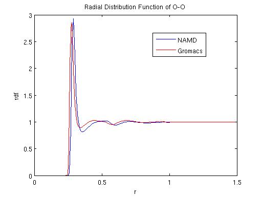
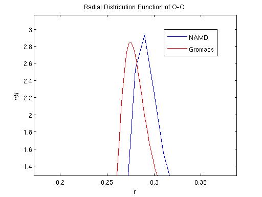
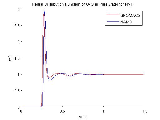
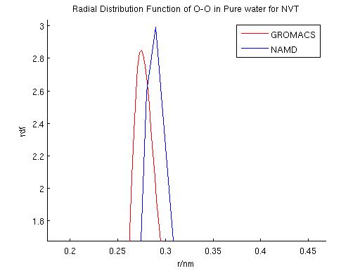
GROMACS and NAMD each adopts different temperature control schemes: GROMACS mainly uses Nose-Hoover and Berendsen thermostat while NAMD mainly uses Langevin dynamics or temperature coupling scheme. We performd NVT simulations using each of these temperature control schemes to compare their effects. Specifically, a first comparison was performed to evaluate the effect of damping coefficients in the simulation result using langevin dynamics. The fluctuation in total energy, temperature and radial distribution function were compared. Diffusion coefficients were also calculated and compared among the different schemes. A second comparison was performed among the three different temperature control schemes.

The effect of damping effects in Langevin Dynamics using TIP3P water model is summarized in Table. 3. It can be seen from Table. 3 that damping affects the diffusion of water dramatically. This can be interpreted from the equation of motion as shown above. The damping coefficient $\gamma$ determines how much friction an atom in the system will experience. The larger the $\gamma$ is, the more friction the sytem will experience. If the langevin dynamics is applied to water molecules, as in our case, you may picture a more and more ``sticky'' water when $\gamma$ is getting larger. In fact, if $\gamma$ is too large, the system will migrate from the inertia regime to the non-inertia regime, and obeys the rules of Brownian dynamics (http://en.wikipedia.org/wiki/). Therefore, $\gamma$ has to be chosen with caution if one's aim is to use Langevin dynamics to control the system temperature. It is noteworty that the experimental value for water diffusion is $\sim 2.3\times10^{-5} cm^2/s$, therefore, using damping coefficient of 5/ps best reproduces the experimental result.

For different temperature control scheme, we have the following three cases, (1) Langevin dynamics with damping coefficient $\gamma$=5/ps (2) Nose-hoover thermostat with $\tau$=0.1 ps (3) Berendsen thermostat with $\tau$=0.1 ps As shown in Table. 5, different temperature control schemes can achieve similar results with well-chosen parameters.

Compare TIP3P and SPCE water models

Although TIP3P is one of the most commonly used water models in MD simulations, various other water models are available, i.e., SPC, SPCE, TIP4P, TIP5P, etc. These different water models may each reproduce the experimental values of different properties of water. Therefore, we extended our simulations and compared the performance of two different water models, TIP3P and SPC. It can be seen from Table. 4 that the two models SPCE and TIP3P appear to have similar dynamic properties. At last, we move on to the water+ion system. As summarized in Table. 6 to Table. 8, for different force field, GROMACS and NAMD gave similar results.

Table 1: NVE zero point

	GROMACS	NAMD
Water Modle	TIP3P	TIP3P
D ( $10^{-5} cm^2/s$)	4.9799 (+/- 0.0012)	5.278 (+/-0.012)

Figure 1: Radial distribution function of water in NVE simulations using GROMACS and NAMD.

Figure 2: Detailed radial distribution function of water in NVE simulations using GROMACS and NAMD.

Figure 3: Radial distribution function of water in NVT simulations using GROMACS and NAMD.

Figure 4: Detailed radial distribution function of water in NVT simulations using GROMACS and NAMD.

Table 2: NVT zero point

	GROMACS	NAMD
Water Modle	TIP3P	TIP3P
Temperature control	Langevin ($\gamma$=5)	Langevin ($\gamma$=5)
D ( $10^{-5} cm^2/s$)	2.5676 (+/-0.00009)	2.769 (+/-0.002)

Table 3: The effect of damping coefficient on water dynamics

	GROMACS	NAMD
$\gamma$=1	4.0702 +/- 0.1798	4.259 +/- 0.025
$\gamma$=5	2.3815 +/- 0.1998	2.769 +/- 0.002
$\gamma$=10	1.9401 +/- 0.0403	1.958 +/- 0.003

Table 4: Comparison of the two water models: SPCE vs. TIP3P

	SPCE	TIP3P
D ( $10^{-5} cm^2/s$)	2.3815 +/- 0.1998	2.5467 (+/- 0.0783)

Table 5: Comparison of different temperature control schemes

	D ( $10^{-5} cm^2/s$)
Langevin	2.5467 (+/- 0.0783)
Berendsen	2.5454 (+/- 0.1814)
Nose-hooever	2.4181 (+/- 0.2624)

Table 6: Water diffusion coefficient in water-ion system

Package	Temperature control scheme	Water model	D ( $10^{-5} cm^2/s$)
NAMD	Langevin ($\gamma$=5)	tip3p(namd)/charmm	2.2247 (+/-0.0015)
GROMACS	Berendsen	spce (gromacs)	2.3026 (+/- 0.00027)
GROMACS	Berendsen	spce (reference)	2.4140 (+/- 0.00006)
GROMACS	Nose-Hoover	spce (gromacs)	2.3235 (+/- 0.00024)
GROMACS	Nose-Hoover	spce (reference)	2.4362 (+/- 0.00036)

Table 7: Na$^+$ diffusion coefficient in water-ion system

Package	Temperature control scheme	Water model	D ( $10^{-5} cm^2/s$)
NAMD	Langevin ($\gamma$=5)	tip3p(namd)/charmm	0.8200 (+/-0.0250)
GROMACS	Berendsen	spce (gromacs)	0.9194 (+/- 0.00120)
GROMACS	Berendsen	spce (reference)	1.3675 (+/- 0.00069)
GROMACS	Nose-Hoover	spce (gromacs)	1.0353 (+/- 0.00021)
GROMACS	Nose-Hoover	spce (reference)	1.2700 (+/- 0.00033)

Table 8: Cl$^-$ diffusion coefficient in water-ion system

Package	Temperature control scheme	Water model	D ( $10^{-5} cm^2/s$)
NAMD	Langevin ($\gamma$=5)	tip3p(namd)/charmm	1.1125 (+/-0.0130)
GROMACS	Berendsen	spce (gromacs)	1.3300 (+/- 0.00064)
GROMACS	Berendsen	spce (reference)	1.6091 (+/- 0.00100)
GROMACS	Nose-Hoover	spce (gromacs)	1.3517 (+/- 0.00050)
GROMACS	Nose-Hoover	spce (reference)	1.4956 (+/- 0.00061)

Appendix I

Simulation parameter

Water Box: 3X3X3 nm$^3$

Number of Atoms: 2685

Density: 991.637 (g/l)

Time-step: 1fs

Electrostatic algorithm:

Long range: PME

Short range: cutoff at 1.0 nm

van der Waals interaction:

switch radius: 1.0 nm cutoff radius: 1.2 nm

Appendix II

Three water models The simple point charge (SPC) model is a three-site model (Berendsen et al., 1987). It consists of a tetrahedral water model with an OH distance of 0.1 nm, H-O-H angle of 109.47$^o$, point charges on the oxygen and hydrogen positions of -0.82e and +0.41e (electronic charge units), respectively, and a Lennard-Jones interaction on the oxygen positions given by

$$V_{LJ} = - (\frac{A}{r})^6 + (\frac{B}{r})^{12}$$

where A = 0.37122 (kJ/mol)1/6· nm and B = 0.3428 (kJ/mol)1/12· nm. However, the center of mass coincides with the oxygen atom for the SPC model.

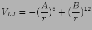
The extended simple point charge (SPC/E) model is characterized by three point masses with O-H distance of 0.1 nm, H-O-H angle equal to 109.47$^o$, charges on the oxygen and hydrogen equal to -0.8476 e and +0.4238 e, respectively, and with Lennard-Jones parameters of oxygen-oxygen interaction according to equation (11.2) (A = 0.37122 (kJ/mol)1/6· nm and B = 0.3428 (kJ/mol)1/12· nm) (Berendsen et al., 1987). The SPC/E model has a dipole moment of 2.35 D. The diffusion constant is improved considerably compared to the SPC model. The agreement of the radial density distribution with experiment is somewhat better for the SPC/E model than for the SPC model (Karniadakis, G., Beskok, A., Aluru, N., Microflows and Nanoflows, Springer, 2005).

Bibliography

Lindahl, E., B. Hess, and D. van der Spoel. 2001.

GROMACS 3.0: A package for molecular simulation and trajectory analysis.
J. Mol. Mod. .

Phillips, J. C., R. Braun, W. Wang, J. Gumbart, E. Tajkhorshid, E. Villa, C. Chipot, R. D. Skeel, L. Kale, and K. Schulten. 2005.

Scalable molecular dynamics with NAMD.
J. Comp. Chem. 26:1781-1802.

George Karniadakis, Ali Beskok, Narayan Aluru, Microflows and Nanoflows Fundamentals and Simulation, Springer, 2005

H. J. C. Berendsen, J. R. Grigera and T. P. Straatsma, J. Phys. Chem. 91 (1987) 6269-6271

Mahoney and Jorgensen (2000). J. Chem. Phys. 112, 8910-8922

Nose, S., A molecular dynamics method for simulations in the canonical ensemble, Mol. Phys., ver 52, pp255-268, 1984

Allen, M.P., Tildesley, D.J., Computer Simulations of Liquids, Oxford Science Publications, 1987

S. Koneshan, Jayendran C. Ransaiah, R. M. Lynden-Bell, S. H. Lee, Journal of Physics and Chemistry B, 1998, 102, 4193-4204

Daan Frenkel and Berend Smit. Understanding Molecular Simulations, Academic Press, 2nd edition, 2001.

About this document ...

This document was generated using the LaTeX2HTML translator Version 2002-2-1 (1.70)

Copyright © 1993, 1994, 1995, 1996, Nikos Drakos, Computer Based Learning Unit, University of Leeds.
Copyright © 1997, 1998, 1999, Ross Moore, Mathematics Department, Macquarie University, Sydney.

The command line arguments were:
latex2html -split 0 report

The translation was initiated by Yi Wang on 2007-05-14