1. Abstract

[Top Of Page]

We will model a neural network in the same style as an Ising Model, with the major difference that all lattice points are connected. Firing and non-firing take the place of spin up an spin down and the connections between the neurons (synapses) are either excitory or inhibitory, and the sum of excitory minus inhibitory neurons determines whether it is firing (positive sum) or non-firing (negative sum). The energy of the configuration of all neurons is found from a sum weighed by the strength of each synaptic connection (the influence of all other neurons determine a neuron's firing state, as described above). All information of the interaction between neurons is stored in this matrix, the synaptic matrix. We assume symmetry in the interactions; the influence of synapse i from synapse j is the same as from synapse j on synapse i.

The firing states can represent a memory of several 2D and 3D shapes, each corresponding to an energy minimum configuration, given through the synaptic matrix. A distorted shape (easily recognizable for a human brain) should then be recalled by the memory through a naive Monte-Carlo simulation. We will begin by allowing each neuron to be influenced by all other neurons in the system, which is realistic for relatively small systems (less than 10⁴ neurons). Primarily, we are interested in seeing how many images we are able to store and recall, modeling neuron decay, and exploring the energy surface of the system.

2. Method

[Top Of Page]

Neurons communicate with each other with electrical signals, the dendrites receive the inputs and the axons transmit the outputs, and the connection from an axon to a dendrite is called synapse. The axons are split into many branches and each neuron has many dendrites, making the system highly interconnected, each neuron transmitting and receiving signals from the order of 10⁴ other neurons. The state of each neuron is defined by its firing rate, that is, the rate by which it is transmitting electrical pulses. The firing rate is a function of the inputs the neuron receives. The synapses can be either excitory or inhibitory, in the former case, if the sending neuron is transmitting with a high firing rate, this will tend to cause a high firing rate of the receiving neuron and in the latter case, a high firing rate will cause a low firing rate of the receiving neuron. The strength of the synaptic connections can differ between all the different neuron. The firing rate is thus a function of all inputs to the neuron. It is approximated as the sum of all inputs through excitory synapses minus the sum of all inputs through inhibitory synapses. This function is very nonlinear and can thus be approximated with a heaviside step function, that is, the neuron is either firing or not firing. It is important to note that it is the firing rate of the neurons that is important, not the timing of the signals, this simplification is justified since it has been empirically shown that firing times of neurons generally are not correlated. Furthermore, the propagation delay in the brain is significantly greater than any delay due to firing rate, and is, on average, constant.

Figure 2.1. A schematic drawing of a neuron. The axon emits the signal and the dendrite collects the signal. One neuron can have up to 10⁴ connections, and is regulated by impulses onto it.

Figure 2.2. The firing rate of a synapse is regulated by both excitory and inhibitory inputs, meaning it is regulated by the presence and lack of signal.

So, what we have is

1. Many on/off devices that are completely interconnected.

2. Whether they are on or off depends on the input from all the other devices.

3. The connections between the devices vary in strength and can be positive (excitory) or negative (inhibitory).

It seems reasonable that this system can be modeled by the Ising model, with each spin corresponding to a neuron and a spin of s=+1 corresponding to the neuron firing and a spin of s=-1 corresponding to it not firing. The modification that is needed is that all spins are now connected instead of just the nearest neighbors. The connection strength is given by the J matrix where the (i,j) element determines how strong the connection from spin i to spin j is. The elements can be positive (ferromagnetic, or in this case, excitory) or negative (antiferromagnetic, or in this case, inhibitory). The total energy of the system is given by

(1)

and he input to neuron i is

(2)

So if this sum is positive (the overall input is more excitory) than inhibitory and it will be energetically favorable that the spin is +1 (firing), vice versa, if the input is negative (overall inhibitory) it will be more energetically favorable that the spin is -1 (not firing). This is analogous to the Ising model where the Ising spin is determined by the fields (and corresponding exchange energies) determined by the directions of the neighboring spins. The system can be simulated in the same way as the Ising model; by using the Monte Carlo method.

The goal is to get this model to function as a memory, that is, we must be able to store and recall patterns. To do this, the spins can be arranged in a lattice with a side of length L and a spin of +1 can be chosen correspond to a black pixel and a spin of -1 can correspond to a white pixel. An initial pattern is chosen, the energy required to flip the spins are calculated, if it's energetically favorable, the spin is flipped. This corresponds to the Monte Carlo method with a temperature of zero. Thus, the system will go directly to the closest energy minimum, which, if the memory works, is one of the stored patterns. If the two initial patterns are close together, they will likely (depending on the energy landscape) reach the same minimum. An approximate measure of how close together two patterns are is the so called Hamming distance, given by

(3)

where m and n are different patterns, N is the number of spins and the summation is over all spins.

The way of calculating the J matrix used here is

(4)

The total energy will then be

(5)

So if the current state of the network is the pattern m, each term is the sum is 1 which ensures that the energy is at a minimum. To store several patterns, the new J can be taken as the weighted sum of the J matrices for the individual patterns.

(6)

This method is associated with Hebb and Cooper. It will lead to a symmetric J matrix, in contrast to the real neural network of the brain which is very asymmetric.

Assumptions and simplifications of the model

1. The neuron is modeled as an on/off device, either firing or not.

2. The timing of the signal is taken as having no importance.

3. The J matrix, and thus the interactions between neurons is symmetric.

3. Experimental Methods

[Top Of Page]

3.1 Understanding Spin Glass

In the process of testing for the maximum number of stored letters, it quickly became apparent that after a certain point the interaction matrix became diluted and would no longer recognize unique images. At this point, it was noticed that many energetically favored equilibrium configurations were composites of many of the letters stored. For example, when storing capitol letters in alphabetical order, letters such as B, D, E, F, etc. all have profound vertical lines oriented along the left edge of the image. If all letters are given the same impact on the interaction matrix, the effect of this left edge will sum together and act as though it is effectively four times more intense.

In order to validate the assumption that these have an additive impact on the interaction matrix, an experiment was run in which all letters of the alphabet were used and the system was allowed to find a low energy stable equilibrium. This equilibrium configuration was then compared to a composite image of all the letters of the alphabet.

3.2 Letter Identification

It is also pertinent to determine how the number of stored patterns or letters affects the chances of identifying an image. To do this, an image of the letter A was loaded and then randomized with a specified percent of randomization between 10% and 100%. Then, for each configuration of random initialization, the monte carlo ising simulation was run using twenty different random seeds and the percentage of the total simulations in which the initial letter A was recognized was recorded.

3.3 Letter Initial Randomization and "Brain Damage"

We are also interested in how initial randomization affects the number of images able to be stored and found again in the J-matrix. Starting with the letter A, and adding letters in alphabetic order, the maximum percentage of randomization while still being able to recall the image was found. How different amounts of brain damage (corresponding to setting some (randomly chosen) percent of J-matrix values to 0) affected this was also investigated. The image size was a constant 40x40 pixels, and the same seed for the random numbers in the MC loop was used for all tests.

3.4 Initial Randomization and Image Size

The same experiment as above was conducted, but now image sizes of 20x20, 40x40, 60x60 and 80x80 pixels were used. Thus, we want to see how different image size affects the number of letters we are able to store. The seed used here was different than the one for testing brain damage, and this explains slightly different values between the 40x40 curve in this image in the last (the "Brain Damage" plot).

3.5 Sensitivity to Initial Spin Damage with Orthogonal Images, Effect of Restricted Interactions Matrix Measurements

In order to minimize the risk for spin glass, the patterns should be orthogonal, this means that

(7)

for m ≠ n. One way of getting close to orthogonal images is to chose all the spins randomly with a 50 % chance for spin up and spin down. This way many more images can be stored in the J matrix before spin glass sets in. If a neural net is to be made out of an integrated circuit, it is preferable if the J-elements are restricted to +1 or -1. To test the effect of this restriction, the maximum initial spin damage that still converge to the initial image for different numbers of stored orthogonal images was found for L = 20, see Fig. 4.5. The "A" pattern was taught, a long with the specified number of orthogonal patterns, the damaged A was then used as the initial pattern.

3.6 Spin Glass with Orthogonal Patterns, Effect of Restricted Interactions Matrix Measurements

The maximum number of stored orthogonal patterns for different sizes of patterns was investigated, with and without restriction in J, see Figure 1. the "A" pattern was taught along with the specified number of orthogonal patterns, the undamaged A was used as the initial pattern.

3.7 Hamming Plots

From the equations in the introduction regarding the Hamming distance, a measure of how similar two images are based on the number of spins in each configuration, we attempt to calculate energy surfaces showing the different minima corresponding to the stored images. The reference image used was a completely black image, meaning all the spins have value -1.

4. Analysis

[Top Of Page]

4.1 Spin Glass

In comparing the composite image with the experimental output, it quickly became apparent that the equilibrium configurations found after glassing of the interaction matrix were related to a weighted sum of the images stored. Specifically, it should be noted that there is a strong vertical linear region on the left side where letters such as B, D, E, F, etc. all have vertical character.

From this, it can be concluded that the spin glass is caused primarily by having repeated character between letters which weight the interaction matrix too strongly toward particular patterns.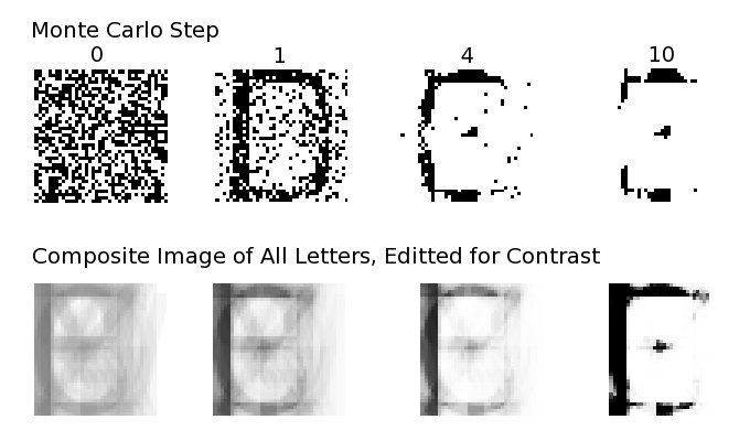

Figure 4.1. (Top) Monte Carlo simulation output at notable steps. (Bottom) A composite image of all letters overlayed ontop one another, adjusted for brightness and contrast to correspond to montecarlo annealing.

4.2 Letter Identification

After plotting the percentage of times the initial image was identified against the number of images stored, it appeared that spin glass for letters appears once eight letters have been stored (in alphabetical order). With 10% initial randomization, the letter was almost always identified until eight letters were stored. Presumably, at this point, the local energy minimum for the letter A was disrupted enough by the other stored images that there ceased to be any sort of minimum to keep the pattern from being converted to a spin glass configuration. This was true for increasing randomization up to about 70% randomization upon initialization, seeing only a slight decrease in the number of letters stored before the letter A was unidentifiable. This is most likely because the randomness imparted onto the letter initially was great enough to overcome the energy barrier between it and alternative configurations. With 90% initial randomization, this trend becomes even more profound, showing relatively low probabilities of identifying the initial configuration. This is because the image is essentially random, and will find the nearest local minimum. For this trial, especially for less than five total stored images, the initial image would settle on another stored image instead of the spin glass, composite image as seen for lower percent initial randomization. This suggests that at high initial randomization, the initial configuration is random enough to overcome energy barriers to other images' local minimum, whereas with low initial randomization, a large number of initial images were needed to pull down the barriers restricting the initial image's transitions.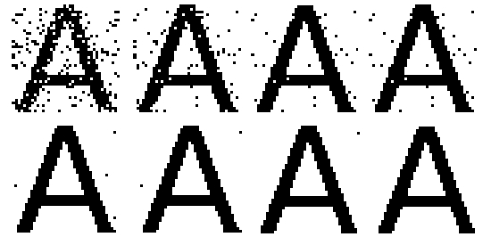

Figure 4.2. An example of the output from the monte calro step. In this example, the intial configuration is an A with 20% randomly oriented spins. In this trial, the simulation falls into a stable A equilibrium configuration.

4.3 Initial Randomization and Brain Damage

The upper limit for images we are able to store was 7, and increasing the brain damage rapidly degrades this number. The maximum percent initial randomization in the input "A" hardly changes for few images stored, and saturates at about 97%. This is to be expected, since every spin is connected to each other - at few images, not many have to be in the correct spot in order to find the image. When more images are stored, a higher proportion have to already be in the correct place, as the bias away from the wished configuration is larger. Attempts to flip the spins will be strongly influenced by the spins that are already in the correct place, and the effect of the random spins will cancel each other out.

The randomization allowed decreases with increased brain damage, as is to be expected. 1% damage has a large effect; there is a pronounced drop in allowed randomization, although the number of images stored remains the same. For 30%, we are only able to recall 5 images as opposed to the usual 7. We did not collect enough data in order to really quantify its effect (or properly estimate any errors), but there seems to be a linear trend in how many images we are able to store compared to the % brain damage. Compare to the number of images we are able to store at 100% of the values in the J-matrix intact (7 images, no brain damage) to some smaller % of intact J-matrix values: 7*70% = 4.9, 7*80% = 5.6 and 7*90% = 6.3. After rounding, these values correspond exactly to the number of images we were able to store with damage. As we are randomly deleting some proportion of the values in the J-matrix, this linearity is not very surprising, as one of the parameters determining how many images can be stored is the size of the J-matrix (the second is the orthogonality of the images).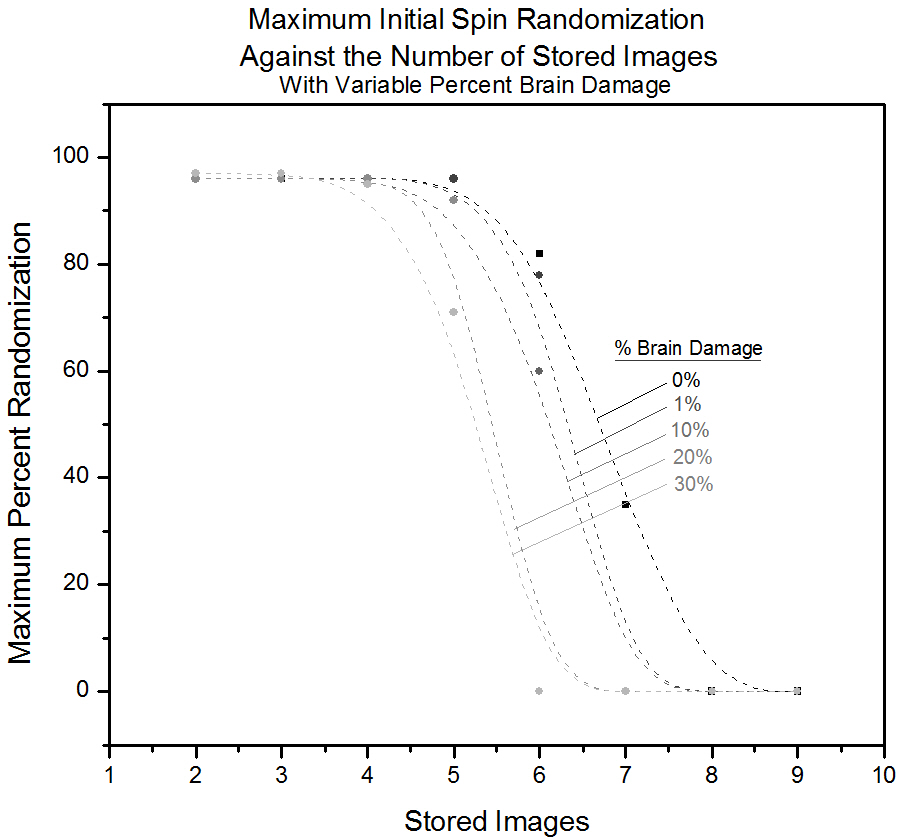

Figure 4.3. A plot depicting the maximum initial randomization which still allows for the desired initial configuration to be determined after the interactions matrix has been configured for the corresponding number of images. With increasing "brain damage" the number of stored images which can be reasonably expected to be distinguishable decreases.

4.4 Initial Randomization and Image Size

As can be seen from the plot, we were not able to store more than 7 images for 60x60 and 80x80 pixels, the same as for 40x40. Although the J-matrix increases in size, the degree of orthogonality of the images is still exactly the same, imposing an upper limit to the number of images we are able to store. That we are not able to store 7 images for 60x60 is an oddity that is probably explained from a small variety in the input images used. We made images of letters from scratch at different pixel sizes, and slightly different centering seems to have a huge effect. This shows the large sensitivity to spin placement, and that we are not able to recall shapes (methods similar to maximum entropy techniques would have to be used). What we should have done was to generate one set of images, and rescale them for all the different dimensions.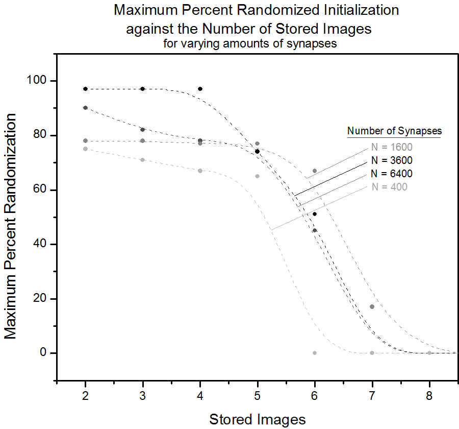

Figure 4.4. A plot depicting the maximum initial randomization which still allows for the desired initial configuration to be determined after the interactions matrix has been configured for the corresponding number of images. The number of synapses is changed giving no clear impact on maximum number of stored images.

4.5 Sensitivity to Initial Spin Damage with Orthogonal Images, Effect of Restricted Interactions Matrix

Restrictive interactions in the J-matrix did not change the system's ability to recall the stored letter with some initial damage appreciably. Since we are simulating only spin up and down, this is not surprising. For any given spin, summing all interactions, it is whether the sum is positive or negative that is important, not the value of the sum itself. Had we simulated in gray-scale (continuous values of our spins), this simplification of the J-matrix would probably have ruined the simulation, as now the strength of the interactions each spin feels becomes important.

It did however have a large influence on the number of stored orthogonal images. The fine-tuning of the J-matrix values becomes very important for a large number of stored orthogonal images, and restricting the values to -1 and +1 means prohibiting the very strong/weak interactions necessary for storing a large amount of images.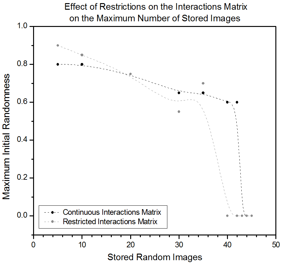

Figure 4.5. A plot depicting the maximum initial randomness on the maximum number of stored images before spin glass occurs using random images. It appears that restricting the J matrix has little affect on the maximum number of images.

4.6 Spin Glass with Orthogonal Patterns, Effect of Restricted Interactions Matrix

It is clear that many more images can be stored if they are orthogonal than when the letters were used, this can be explained by the larger Hamming distance for the orthogonal images which causes the minimas in the energy landscape (between the orthogonal images and the A) to be further apart, thus the patterns don't interfere with one another. Nevertheless, if too many patterns are stored, the minimas will become too crowded together and not very deep; the system will no longer function as a memory. The theoretical limit for when this happens is around 0.13L². This limit is not reached, this can be explained by the fact that the stored patterns are not completely orthogonal and the A is certainly not orthogonal to the other randomly generated patterns.

Not as many patterns can be stored if the J matrix is restricted, the difference is however not very large. It was also found that adding a random component to the J matrix has a larger detrimental effect on the ability to store patterns than on the sensitivity to initial spin damage.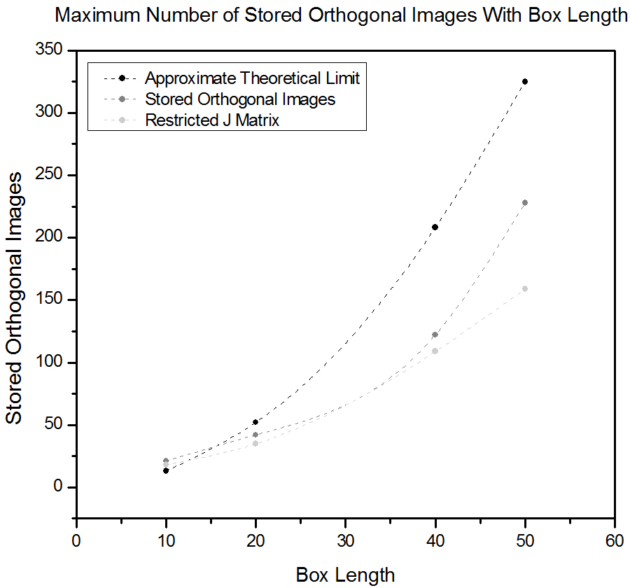

Figure 4.6. A Plot depicting the maximum number of stored orthogonal images while still being able to distinguish the initial configuration.

4.7 Hamming Plots for Letters

For 40x40 pixels images, we stored the letters A, B, C and scanned the energy surface by annealing (starting at some temperature, constantly decreasing, eventually ending up at T=0). In the figure below, each letter correspond to a local energy minima. What is discouraging for our method is the formation of a "spin glass" global energy minimum. As the J-matrix is the sum of the interactions from all the input letters, this is not very surprising, and the spin glass configuration is clearly looks like a mix of all the letters.

We also stored the 8 first letters in the alphabet. This is larger than the number of spin states the system is able remember, and any local minima are too close together. After just a few MC sweeps, the configuration ends up in the spin glass state.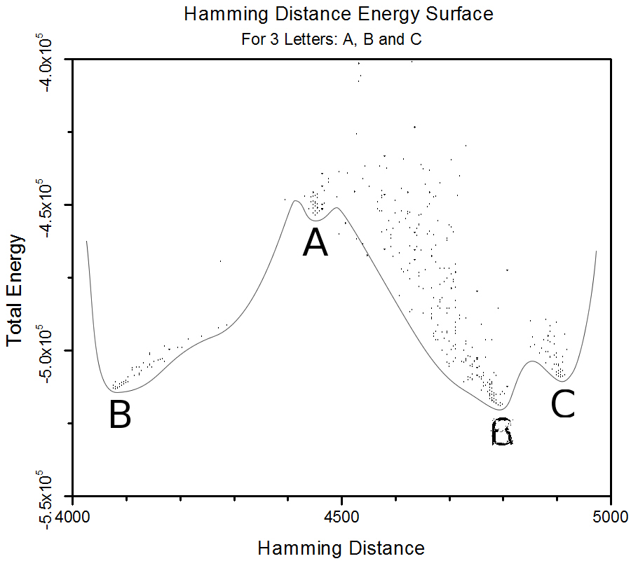

Figure 4.7. A plot depicting the total energy for configurations with varying Hamming distances. Note the apparent energy surface, and the distinct trough for A when there are only 3 letters.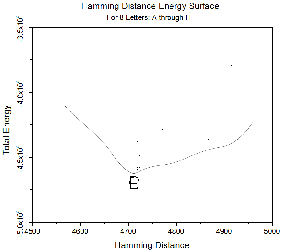

Figure 4.8. A plot depicting the total energy for configurations with varying Hamming distances. Note that the trough for A has been completely overwhelmed by a lower hybrid configuration.

4.8 Hamming Plots for Orthogonal Images

Hamming plots were also made for 20x20 pixel images, using 40 and 60 orthogonal images and the letter A, to see how the energy surface changes compared to only storing letters. The same trend as for only storing letters can be seen, but there is no identifiable spin glass formation for only 40 orthogonal images, as the values in the J-matrix coming from A are very distinct compared to those from the orthogonal images. For 60 images, this changes, and there is a global minima of a spin glass at Hamming distance of about 870.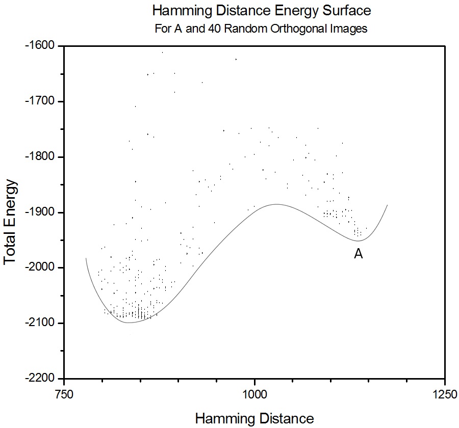

Figure 4.9. A plot depicting the total energy for configurations with varying Hamming distances. Here, A has a distinguished minimum, but a hybrid configuration of orthogonal images produces a more stable state.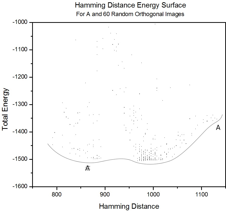

Figure 4.10. A plot depicting the total energy for configurations with varying Hamming distances. Here, A is unstable, and the end configuration is always a spin-glass configuration (depicted).

5. Conclusions and Further Work

[Top Of Page]

We successfully coded a method to store .bmp images as -1 and 1's in a square array, and applied an Ising type Hamiltonian with all spins interacting. Images were able to be stored, and we investigated how damage to the images and the matrix storing the interactions affect the ability to recall images.

Efforts to calculate the J-matrix iteratively, changing random J-values in order to fit the interactions resulting from each image, were also thought about. We reached the conclusion, however, that this would just give us the same overall J-matrix as the hard-coded version we implemented, with some slight randomization.

One of the major obstacles to storing images with this method is that shapes are not recognized; moving the same image around has a large effect on its ability to be recalled. Algorithms including for example maximum-entropy methods would have to be included to fix this issue.

Bibliography

[Top Of Page]

(1) Giordano, Nicholas J. "11.3 Neural Networks and the Brain." Computional Physics. Upper Saddle River, NJ: Prentice-Hall, 1997. 328-45. Print.

(2) Maximum Entropy Image Reconstruction - General Algorithm. Authors: Skilling, J.; Bryan, R. K.. Publication: R.A.S. MONTHLY NOTICES V.211, NO.1, P. 111, 1984