Molecular static study on voids in UO2

Wei Ying Chen

Project report for MSE485

Abstract

Molecular static calculation is done on Schottky defect cluster(voids) in uranium oxide. It is found that there is no maximum size limit on voids in the perspective of enthalpy. A transition from line shape to plane (disk) shape is found as well when number of pairs is beyond 4 in the cluster.

1. Introduction

Voids is important in perspective of mechanical property and fission gas storage of nuclear fuel.

Even though voids have been routinely observed in irradiated materials, it is hard to investigate the early stages of the formation process. Thus, computer simulation can provide a lot of information which is not obtainable from experiment.

Sabochick et. al. [1]calculated large vacancy clusters(10 ~ 40 vacancies) in copper. Transition between dislocation loops and stacking fault tetrahedra is predicted. Similarly, the goal of this project aims at weather there is a maximum size that a void can ever attends thermal-dynamically. If yes, what is the maximum size? What is the most energetically favorable void shape for different sizes. Also, it would be valuable to find the transition point where some kind of shape become more favorable over the other.

MD programs GULP[2] is widely used either in molecular dynamics and molecular static calculations. It was originally designed for fitting the interatomic potential to both energy surface and empirical data. Now it’s been expanded to handle a variety of tasks. This project mainly employed GULP to perform molecular static calculation.

2. Computation method

The basic approach of this project is:

1. Construct perfect uranium dioxide lattice.

2. Put Schottky defects into this perfect lattice according to the shape I want. Shapes   considered will be discussed later.

3. Relax the system to minimize its energy. The strategy to minimize the energy will be discussed later. The potential and potential energy summation technique is also discussed later.

4. Calculate the formation energy. Formation energy is defined as the difference of enthalpy between perfect system and system containing defects.

5. Compare the formation energy per pair of Schottky defect for different size and shape. Make the conclusion according to this.

2-1. Shapes of clusters

 Three types of voids shapes are considered: one dimensional (line), two dimensional (plane) and three dimensional. For each type, the building unit is a single Schottky defect whose oxygen vacancies and uranium vacancy are confined in a [1 1 1] line.

For line shape, Schottky defects are clustered in [1 1 0] direction. That is, the uranium vacancy is put starting from [0 0 0], and then [0.5 0.5 0] then [1 1 0] and so on. Size is considered from 2 to 6 pairs of Schottky defects.

For plane shape, (111) and (11-1) planes are both considered. This is because the angle between Schottky defect and the cluster plane might makes a difference on formation energy. Schottky defects are placed in the plane in a way that the area is minimized. Sizes ranges from 3 to 8 pairs are calculated.

For 3 dimensional case, only triangular pyramid of size four pairs is calculated so far.

2-2. Energy minimization strategy

Defect formation energy is evaluated by Newton-Raphson energy minimization with Mott-Littleton method[8].

2-2-1. Energy minimization

Equilibrium structure is found by searching the minimum of the potential surface. The true minimum, global minimum can be searched via either the Monte Carlo, simulated annealing or genetic algorithms. In this project, I want only to find the local minimum around the defect cluster.

Suppose x is the position vector matrix of the system, then we can expand the internal energy as a Taylor series:

The first derivative is the gradient vector, g. The second derivative matrix is called Hessian matrix, H. If the calculation cut the Hessian term, then only the total energy and the gradient is considered. The gradient is then used to determine the direction of movement. A line search is to determine the magnitude. The above is called the steepest gradient. A more sophisticated algorithm called conjugate gradient[3] was developed to increase the efficient by direct the next step from the previous step.

Instead of expand the energy U to the first order, Newton - Raphson procedure expands U to the second order. The displacement vector ∆x, vector from current position to the minimum energy position can be expressed as:

∆x = - H^-1 g

If the energy surface is harmonic, then we can attend to the minimum in one step. However for the real energy surface, the above expression is just an approximation. So multi-cycles are needed to find the minimum.

The most expensive part in Newton - Raphson method is the inversion of Hessian matrix. To tackle this, Broyden-Fletcher-Goldfarb-Shanno(BFGS) [4]method provides a way to update Hessian matrix so to avoid inverting the Hessian completely each cycle.

In my project, both conjugate gradient and Newton-Raphson are used to optimize the structure. It is found that although conjugate gradient proceed faster cycle by cycle than Newton-Raphson does, conjugate gradient usually can not achieve optimization criteria. So, Newton-Raphson is adopt for most of the calculations. However, when size of the system is increased, the computational cost for New-Raphson grows as N³. The memory resources then become a problem. For the cluster I used, an memory allocation error occurs when system size is beyond 8000 atoms.

2-2-2. Potential

Since UO2 is ionic materials, the usual form of pair potential is the addition of a Buckingham form to  the Coulomb potential.

where r is the distance between i and j.

coulomb interaction is the most important term for total enthalpy. Coulomb energy(potential energy) is hard to calculate for periodic systems because it’s conditionally convergent. In three dimensional situation, the interaction between atoms decay as r ^-1, but the number of interacting atoms increase as 4πr². Thus the energy density contribute to the center atom will increase with radius. The most popular method  to tackle this is the method of Ewald[5]. By requiring neutrality and zero dipole moment, the series of summation become convergent. The Coulomb potential energy is separated into two part, one of which decays fast in real space and the other decays fast in reciprocal space. The resulting electrostatic potential energy is a summation of U^real, U^reciprocal and self-energy of the ion.

where G is reciprocal lattice vector. V is volume of one unit cell(~158.34 ų for UO2 case). η is a parameter that controls the division of work between real and reciprocal space.

For Buckingham term, a bunch of parameter sets(A, ρ and C) are developed to fit uranium dioxides properties like lattice constant or elastic constant. In this project I used the potential developed by Grimes[6]. The basis for Grimes potential were electron-gas calculations and it’s an shell-core type of potential. The parameters are listed in the following Table 1.

Govers [7] used Grimes as well as all other potentials for UO₂ to calculate lattice constant, elastic constant, formation energy, migration energy and volume change due to defects. After comparing all the results, Grimes’ potential is found not overestimate the formation energy. However, since Grimes’ potential is widely used in UO₂ and partially since our group is using Grimes’ potential, I adopt it for a moment. Other potentials should be tested in the future.

Parameters	value	Units
Charges
O shell	-4.4	e
O core	2.4	e
O spring	296.8	eV/Å^2
U shell	6.54	e
U core	-2.54	e
U spring	98.24	eV/Å2
Parameters: O - O interactions
A	108	eV
ρ	0.38	Å
C	56.06	eVÅ^6
Parameters: O - U interactions
A	2494.2	eV
ρ	0.34123	Å
C	40.16	eVÅ^6
Parameters: U - U interactions
A	18600	eV
ρ	0.27468	Å
C	3264	eVÅ^6

Table 1. Parameters for Grimes’ potential

2-2-3. Defect calculation strategy

To find the defect formation energy is equal to find the minimum energy configuration around the defect. There are two strategies: periodic boundary condition( PBC) method and Mott-Littleton method[8]. Both methods are implemented in GULP code.

For PBC, atoms in the cell not only interact with defects inside the cell but also interact with defects in image cell. In order to reduce this effect, the simulation cell size must be large enough. The energy minimization process will then become too time-consuming, especially for Hessian calculation.

On the other hand, Mott-Littleton method is more efficient. The method divides the environment around defect into three regions by two concentric sphere. In the central sphere is where Schottky defects are built. Ions are strongly affected by defects in this region and relaxations are calculated fully. In the closest  shell, the intermediate region, ions are only slightly perturbed. A harmonic relaxation is performed in this region. For the outmost region, which extends to infinity, it is treated as  dielectric medium.

Since Mott-Littleton method converges faster and since my computer resources is limited. I adopt Mott-Littleton method to carry out defect formation energy. Radius of spheres used in this project were 14 and 24 Å. Cut off distance for short range interactions used in the project was 10.4 Å.

3. Results and discussion

The results is summarized in Table 2,3,4,5 and figure 1.

Line # pairs	Formation Energy per pair(eV)
2	5.9081
3	5.486
4	5.28
5	5.158
6	5.075

Table 2. Formation energy per pair of Schottky in line shape

Plane(111) # pairs	Formation Energy per pair(eV)
3	7.2057
4	8.7722
6	7.1431
7	9.2281

Table 3. Formation energy per pair of Schottky in plane shape on (111) plane

Plane(11-1) # pairs	Formation Energy per pair(eV)
3	5.6628
4	4.6498
5	4.7582
6	4.8144
7	4.4413
8	4.4621

Table 4. Formation energy per pair of Schottky in plane shape on (11-1) plane

3D # pairs	Formation Energy per pair(eV)
4	5.7702
6	5.6182

Table 5. Formation energy per pair of Schottky in 3D shape

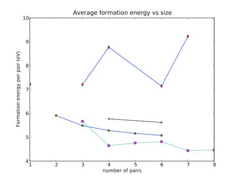Figure 1. A summarized plot of all data points. The line with diamond mark is for plane shape on (111). The line with star mark is for 3D shape. The line with square mark is for plane shape on (11-1). The line with pentagon mark is for line shape.

The calculated formation energy for one single Schottky defect is 7.218 eV. Compared ab initio result 4.1 eV, result from Grimes is overestimated, but in the same order.

For Line shape, the average formation decreases as length increases, implying that cluster can always lower system enthalpy by lengthening itself. Binding energy is also calculated  to be around 2.5 eV and keep steady as size grows. Even though I don’t have too much data points,  I believe the tendency is obvious: There is no limit on the length of line shape voids.

For plane shape, The results are quite interesting and unexpected. Average formation energy for (11-1) plane shows an gradual decline with increasing size but the one for (111) is scattered and ,most importantly, above 7.1 eV. Cluster on (11-1) has a tendency to grow in size whereas cluster on (111) tend to dissolve( or transfer to lower energy configuration).

The reason for this is the relative orientation of Schottky defect and the plane. For (111) case, Schottky defects ( [111] line) is perpendicular to the deposited plane. For (11-1) case, it is tilt more to the deposited plane. The volume occupied for (111) case is more and thus a larger strain energy is caused, which is so large that it becomes unfavorable energetically.

One more thing to notice is the little bulge between size 4 to 7. The slight increasing arises from the broken symmetry of hexagonal shape of the cluster. Formation energy per pair is especially low for complete hexagonal shape.

Lastly, the 3 dimensional case. Because of the limited time and computing power, only two case is done. It seems to have the similar declining trend as line shape and (11-1) plane shape does.

Put them all together, we can conclude that line shape is the most stable shape for size 1 to 3. Starting from size 4, plane shape on (11-1) takes place as most stable configuration. A transition happens between size 3 and 4. Besides, since average formation energy seems to approach a equilibrium value below 7.18 eV, a limit on void size doesn’t exist. Voids can always grow as long as there is sufficient Schottky supply.

4. Reference

[1] M J Sabochick et al 1988 J. Phys. F: Met. Phys. 18 349 (1988)

[2] J. D. Gale, A. L. Rohl, Mol. Simul. 29 (2003) 291

[3]W.H. Press, S.A. Teukolsky, W.T. Vetterling, and B.P. Flannery. Numerical recipes in Fortran: The art of scientific computing. Cambridge University Press, 1986.

[4] D.F. Shanno. Conditioning of quasi-newton methods for function minimization. Math. Comput., 24:647–656, 1970.

[5]P.P. Ewald. Die berechnung optischer und elektrostatisher gitterpotentiale. Ann. Phys., 64:253–287, 1921.

[6]R. W. Grimes, C. R. A. Catlow, Philos. Trans. R. Soc. Faraday Trans. 86 (1990)

[7]K. Govers, S. Lemehov, M. Hou, M. Verwerft, J. Nucl. Mater. 366 (2007) 161

[8]N.F. Mott, M.J. Littleton, Trans. Faraday Soc. 34(1938)