Path Integral
CSE 485
Tom Galvin
Table of Contents
1. Helium
2. Introduction
to Path Integral Monte Carlo
4. Testing
5. Results
6. Conclusion
7. References
8. Links
9. Presentation
The low mass of 4He
and the fact that it behaves as a boson makes it an ideal system to demonstrate
quantum boson effects. Liquid helium-4
is a well studied system [1]. It is a liquid
below 5.2 K and under 25 atm of pressure. At approximately 2.17 K, a transition occurs
between the regular liquid and superfluild
states. This is known as the lambda
transition, so called because of the characteristic shape of the heat capacity
curve as a function of temperature. The
goal of my project is to spot the lambda transition by looking at the specific
heat [2].
As a rule of thumb, τ
< .02 (τ will be described in the next section) to accurately simulate
a Leonard-Jones potential with a free particle kinetic action. This can involve up to 40 time slices at the
temperature of the lambda transition.
Calculations involving even a few particles and such a large number of
time slices are computationally infeasible with the computing power of a home
computer. Researchers circumvent this
problem by analytically solving the two-body density matrix. This enables them to write a more accurate
kinetic action which in turn allows larger time slices. However for this project, a simplified model
of helium is assumed. The helium atoms
will be treated as a hard sphere with a radius of 2.14 angrstrom
[3]. This model will hopefully capture
the essential physics, though the exact temperature and shape of the lambda
transition will be off.
To the author’s knowledge no
hard sphere PIMC simulation of 4He has been published. However this is probably due to the fact that
with freely downloadable
C code, much more accurate simulations can be done on a personal computer.
Path Integral Monte Carlo (PIMC)
Imaginary time path integral
monte carlo (PIMC) is a
method of computing thermal averages of highly quantum systems.
For the following
discussion, take definitions:
N – the number of particles
in the system
M – the number of steps in
the a PIMC ring
T – the temperature of the
system
R – vector of 3N coordinates
of all particles
![]() —the potential energy operator
—the potential energy operator
V—the potential action
![]() —the kinetic energy operator
—the kinetic energy operator
K—the kinetic action
m—the mass of each particle
ρ—the thermal density
matrix
![]()
![]()
![]()
The thermal expectation for
any operator can be written as:
![]()
While this identity is
wonderful for theoreticians, a method is needed to evaluate the integral on the
right. The basis for PIMC comes from the
following identity:
![]()
which is exact. By making use of the above identity M times, we
get:
![]()
Or upon inserting the
identity M times:
![]()
Although this may appear
more complicated, the above integral can be evaluated with monte
carlo sampling techniques. In PIMC parlance, each inserted R is
known as a ‘bead’ or ‘time slice’. As M
increases, τ decreases, which means the temperature is going up. As the temperature rises, particles behave
more classically. Therefore if enough
steps are used, we can use a semiclassical
approximation for the density function.
We start with the following, identity, which is known as Trotter’s
formula:
![]()
Then we seek semiclassical approximations for ![]() and
and
![]() . At this point it is
customary to switch from density matrices into actions. The action is defined as:
. At this point it is
customary to switch from density matrices into actions. The action is defined as:
![]()
![]()
![]()
Using some fancy
derivations, we obtain the primitive actions [5] :
![]()
![]()
There is of course one more
degree of freedom: permutations. States
in which the coordinates of the particles are switched but the positions remain
the same are indistinguishable. Particle
permutations result in bosons having a tendency to bunch together. A monte carlo move must be included to flip sections of the paths.
Calculating
Observables
Observables can be divided
into two categories: those which are diagonal in the position basis, and those
which are not. Diagonal observables
include energy, pressure, pair correlation and conductivity. These properties are measure with closed loop
paths. Off diagonal properties are
calculated with non-closed paths. Slight
modifications to the procedure discussed above are needed to calculate
off-diagonal properties. Because we are
not interested in these properties, they will not be discussed.
In this section common PIMC
moves will be discussed. Moves which
raise the total action are automatically accepted. The local nature of the moves means one does not
have to recalculate the action of the entire system after every move. Rather it is possible to just calculate the
changes in the action that result from the moves.
Single Particle
In this move single time
slice of one particle is randomly displaced and the change in action is
calculated. Naively, this is the only monte carlo move necessary for
distinguishable particles. Additional
moves are typically used to sample phase space more rapidly.
Displacement
Moving one time slice of a
particle at a time inefficiently moves the center of mass of the entire
path. The displacement move can be
introduced to fix this. In this move all
particles are uniformly displaced in the direction of a single vector.
Rotation
This move is similar to the
displacement move, in that all beads of a particle are moved at once. The beads are rotated along a random angle of
the center of mass of the path.
The Bisection Move
In this move a whole section
of a path is resampled. A section of the
path consisting of 2k -1 points is first removed from the path. The midpoint of the missing section is then
sampled. One each side of the resampled
midpoint, there will be two 2k-1 -1 gaps in
the path. The midpoints of these two
gaps are then sampled. This process will
continue until all of the slices have been resampled. The move is accepted or rejected as a
whole. Because the largest path is
resampled first, less time will be spent generating random paths that will be
rejected anyway.
Permutation
All moves discussed thus far
have focused on moving particles around the space. The permutation move is fundamentally
different type of move. It is necessary
to simulate bosons at low temperature.
Consider two nearby
particles A and B, each with time slices indexed by n. When going from slice n to n+1,
whether A(n)àA(n+1)
and B(n)àB(n+1) or A(n)àB(n+1) and B(n)àA(n+1) are indistinguishable situations. If A and B are permuted, the effect is join
of the paths if they are on separate paths, or to break a path if they are
already on the same path.
The code for this project
was implemented in Matlab. Two files were written for this project PIMC2.m and FindCv.m. PIMC2 performs the actual simulation. FindCv is simply a
script to help summarize the results.
Random numbers were generated via the Mersenne
Twister algorithm built into Matlab.
The simulation file begins
with the definition of all of the constants which will be needed in the
calculations. Atomic units have been
used, which are not the typical units of the liquid helium community. The atoms are initialized in a simple cubic
lattice, with all time slices at the same spot.
The approximation of a hard
sphere potential allows several simplifications in programming. First, the potential energy is always
zero. Any move which would bring two
atoms too close together would be rejected.
Next, the atoms behave as free particles when they are far enough
apart. This makes the primitive action
almost exact. Hence fewer time slices
can be used. As a result of the small
number of time slices, it was only necessary to implement the single particle
move and the permutation move. Even with
just these two moves, the correlation time remains reasonable.
In most PIMC algorithms, the
R vectors are sorted by which particle they belong. By convention all permutations take place at
the same time slice. This requires an
extra
The single particle move was
straightforward. A particle was moved
randomly at one time slice. The change
in kinetic action was monitored, and the code checked for collisions. The acceptance ratio varied from .6 to .07
depending on the temperature. The
permutation move was much more difficult.
There is a lot of bookkeeping to keep track of which connection goes
where. The code handles three cases: 1.
Where a particle attempts to permute with itself. In this case nothing is done. 2. Where two particles in the same path are
permuted. This has the effect of
breaking the path. First the code finds
an empty spot in the array to place the new path. It is broken off and the change in kinetic
action checked. 3. Two particles on different paths are
permuted. In this case the paths are
joined. Room is made for one path to fit
in the middle of the other.
Before the simulation
begins, the kinetic action is set to zero.
This is because all the beads for each particle are in the same
place. Each function that can change the
kinetic action returns to the main loop by how much the kinetic action is
changed. At the end of the run the
kinetic action is scaled and offset to produce the energy.
The code after the main loop
automatically computes the mean, standard deviation, autocorreation
time, and the error of the mean. The
autocorrelation time is estimated using Matlab’s xcorr function.
After PIMC2 exits, further processing is done to calculate C_v. The derivative
of E with respect to T is estimated to the fourth order via
Optimizations
The first rather obvious
optimization to the code is that the kinetic action is not computed ab-initio for every run.
Instead the action is computed once, and we keep track of the change in
the action each cycle. The kinetic
action is much easier to compute than the interaction potentials. In each single particle move, the change in
energy from the action is first computed.
Before computing the pair potential, we look to see if the move would
have been rejected on the basis of the change in kinetic action anyway. This saves us from having to compute the pair
potential in moves which would have been rejected anyway. It was accomplished using the
short-circuiting feature of Matlab or functions.
The use of ‘if’ statements was avoided as much as possible because they slow down the processor. For ease of maintenance, each pass of the monte carlo code still required several function calls. In C, this could be fixed by using the #inline command.
Before simulations were run, several tests were performed to determine
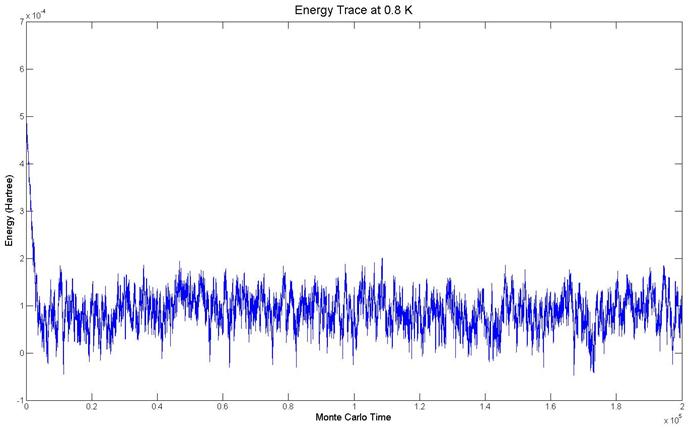
whether the output would in general be reasonable. The first and most obvious test of the code
is to determine whether the energy converges and appears to have a finite
divergence. The energy trace for the
system with 8 beads at 0.8 K is shown below.
It is typical of energy traces observed.
No spikes appear in the output and it appears converged.
In the limit that the box is
very large, the particles essentially do not interact. Classically this is known as an idea
gas.. The energy should be:
![]()
This line is drawn in red on
the plot below.
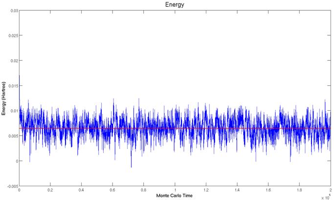
The simulated and calculated values agree well. Specifically, the energy predicted by the simulation was Esim = 2.573e-3 Hartree while the ideal gas law predicts EIGL = 2.565e-3 Hartree. This is within the standard error of the simulation σ = 2.093e-5 Hartree.
More simulations were done performed in the low density ideal gas limit. The outputs are shown below:
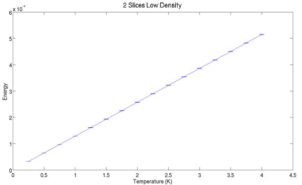
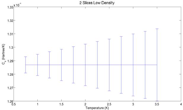
The energy varies linearly
with temperature and the heat capacity is constant as expected. The theoretical value for the heat capacity is
CV = 1.287e-4 Hartree/K, which
agrees well with the lower plot.
Further validation included
stepping through the code line by line to verify that the code behave as
expected.
The lambda transition occurs
at a temperature of around 2.1 K with an atomic volume of around (3.6 A)3
[5]. For my simulations, the temperature
was swept. The box size was chose to give
each helium atom (4.46 A)3 of
space. The density was not higher
because if the density gets too high, the particles have nowhere to move. They may not be able to reach equilibrium
within the simulation time if they are packed in too tight. The simulation used 27 particles. This number can be easily initialized on a
cube. More particles would have made the
heat capacitance transitions sharper, but computing resources were limited.
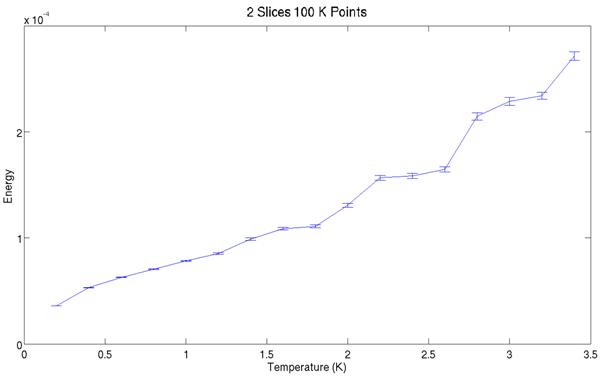
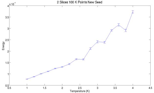
The two plots above show the
simulated energy for two slices at various temperatures. Note they do not cover the same range in
temperature. Between the graph all that was varied was the random number generator
seed for starting the simulation. Close
examination reveals the two graphs do not predict identical energies at a given
temperature. The simulation may not be
behaving ergodically. It could be that the atoms are packed too
tight in the simulation and certain phase space configurations are thus
inefficiently sampled.
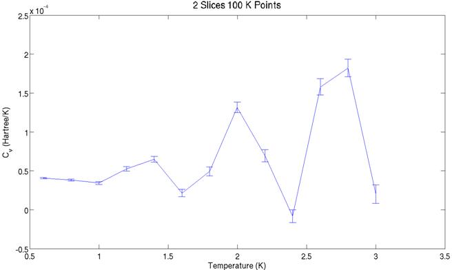
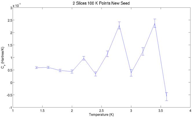
The two graphs above show
the heat capacity values derived from the energy graphs further above. They share a similar structure, but the peaks
are offset. The aforementioned non-ergodicity
is most likely to blame for this. Significantly
increasing the number of
![]() The
simulations have been shown to reproduce classical results.
The
simulations have been shown to reproduce classical results.
![]() The
system may be behaving non-ergodically at high
densities. A change in the random number
seed produced visible changes on the energy graph. This could be overcome by increasing the run
time of the simulations to give them more time to sample phase space. This is not currently possible due to limited
computing resources.
The
system may be behaving non-ergodically at high
densities. A change in the random number
seed produced visible changes on the energy graph. This could be overcome by increasing the run
time of the simulations to give them more time to sample phase space. This is not currently possible due to limited
computing resources.
![]() Originally
I was hoping to leverage the SIMD capabilities of Matlab
to make the code run faster despite being written in an interpreted
language. However, there were relatively
few opportunities to vectorize mathematical
operations. As a result, the code is
quite slow compared to what I’m sure is possible with C. Compiling may have improved performance. Uncompiled Matlab code is unsuitable for this type of simulation.
Originally
I was hoping to leverage the SIMD capabilities of Matlab
to make the code run faster despite being written in an interpreted
language. However, there were relatively
few opportunities to vectorize mathematical
operations. As a result, the code is
quite slow compared to what I’m sure is possible with C. Compiling may have improved performance. Uncompiled Matlab code is unsuitable for this type of simulation.
[1] D. M. Ceperly. Path
Integrals in the theory of condensed helium.
Rev. Mod. Phys., 67(2):279, April 1995.
[2] K. Kittel
and H. Kroemer Thermal Physics.
[3] M. H. Kalos, D. Levesque, and L. Verlet. Phys. Rev. A., 9, 2178 (1974).
[4] K. Esler.
“Advancements in the path integral monte carlo method for many-body quantum systems at finite temperature,”
Ph.D. thesis,
[5] R, P. Feynman. Space-time approach to non-relativistic
quantum mechanics. Rev. Mod. Phys.,
20:367, April 1948..