LU Decomposition for Solving Linear Equations
Learning objectives
- Describe the factorization \({\bf A} = {\bf LU}\).
- Compare the cost of LU with other operations such as matrix-matrix multiplication.
- Identify the problems with using LU factorization.
- Implement an LU decomposition algorithm.
- Given an LU decomposition for \({\bf A}\), solve the system \({\bf Ax} = {\bf b}\).
- Give examples of matrices for which pivoting is needed.
- Implement an LUP decomposition algorithm.
- Manually compute LU and LUP decompositions.
- Compute and use LU decompositions using library functions.
Forward substitution algorithm
The forward substitution algorithm solves the linear system \({\bf Lx} = {\bf b}\) where \({\bf L}\) is a lower triangular matrix.
A lower-triangular linear system \({\bf L}{\bf x} = {\bf b}\) can be written in matrix form:
\[\begin{bmatrix} \ell_{11} & 0 & \ldots & 0 \\ \ell_{21} & \ell_{22} & \ldots & 0 \\ \vdots & \vdots & \ddots & 0 \\ \ell_{n1} & \ell_{n2} & \ldots & \ell_{nn} \\ \end{bmatrix} \begin{bmatrix} x_1 \\ x_2 \\ \vdots \\ x_n \end{bmatrix} = \begin{bmatrix} b_1 \\ b_2 \\ \vdots \\ b_n \end{bmatrix}.\]This can also be written as the set of linear equations:
\[\begin{matrix} \ell_{11} x_1 & & & & & & & = & b_1 \\ \ell_{21} x_1 & + & \ell_{22} x_2 & & & & & = & b_2 \\ \vdots & + & \vdots & + & \ddots & & & = & \vdots \\ \ell_{n1} x_1 & + & \ell_{n2} x_2 & + & \ldots & + & \ell_{nn} x_n & = & b_n. \end{matrix}\]The forward substitution algorithm solves a lower-triangular linear system by working from the top down and solving each variable in turn. In math this is:
\[\begin{aligned} x_1 &= \frac{b_1}{\ell_{11}} \\ x_2 &= \frac{b_2 - \ell_{21} x_1}{\ell_{22}} \\ &\vdots \\ x_n &= \frac{b_n - \sum_{j=1}^{n-1} \ell_{nj} x_j}{\ell_{nn}}. \end{aligned}\]The properties of the forward substitution algorithm are:
- If any of the diagonal elements \(L_{ii}\) are zero then the system is singular and cannot be solved.
- If all diagonal elements of \({\bf L}\) are non-zero then the system has a unique solution.
- The number of operations for the forward substitution algorithm is \(O(n^2)\) as \(n \to \infty\).
The code for the forward substitution algorithm to solve \({\bf L x} = {\bf b}\) is:
import numpy as np
def forward_sub(L, b):
    """x = forward_sub(L, b) is the solution to L x = b
       L must be a lower-triangular matrix
       b must be a vector of the same leading dimension as L
    """
    n = L.shape[0]
    x = np.zeros(n)
    for i in range(n):
        tmp = b[i]
        for j in range(i-1):
            tmp -= L[i,j] * x[j]
        x[i] = tmp / L[i,i]
    return x
Back substitution algorithm
The back substitution algorithm solves the linear system \({\bf U x} = {\bf b}\) where \({\bf U}\) is an upper-triangular matrix. It is the backwards version of forward substitution.
The upper-triangular system \({\bf U}x = b\) can be written as the set of linear equations:
\[\begin{matrix} u_{11} x_1 & + & u_{12} x_2 & + & \ldots & + & u_{1n} x_n & = & b_1 \\ & & u_{22} x_2 & + & \ldots & + & u_{2n} x_n & = & b_2 \\ & & & & \ddots & & \vdots & = & \vdots \\ & & & & & & u_{nn} x_n & = & b_n. \end{matrix}\]The back substitution solution works from the bottom up to give:
\[\begin{aligned} x_n &= \frac{b_n}{u_{nn}} \\ x_{n-1} &= \frac{b_{n-1} - u_{n-1n} x_n}{u_{n-1n-1}} \\ &\vdots \\ x_1 &= \frac{b_1 - \sum_{j=2}^n u_{1j} x_j}{u_{11}}. \end{aligned}\]The properties of the back substitution algorithm are:
- If any of the diagonal elements \(U_{ii}\) are zero then the system is singular and cannot be solved.
- If all diagonal elements of \({\bf U}\) are non-zero then the system has a unique solution.
- The number of operations for the back substitution algorithm is \(O(n^2)\) as \(n \to \infty\).
The code for the back substitution algorithm to solve \({\bf U x} = {\bf b}\) is:
import numpy as np
def back_sub(U, b):
    """x = back_sub(U, b) is the solution to U x = b
       U must be an upper-triangular matrix
       b must be a vector of the same leading dimension as U
    """
    n = U.shape[0]
    x = np.zeros(n)
    for i in range(n-1, -1, -1):
        tmp = b[i]
        for j in range(i+1, n):
            tmp -= U[i,j] * x[j]
        x[i] = tmp / U[i,i]
    return x
LU decomposition
The LU decomposition of a matrix \({\bf A}\) is the pair of matrices \({\bf L}\) and \({\bf U}\) such that:
- \({\bf A} = {\bf LU}\)
- \({\bf L}\) is a lower-triangular matrix with all diagonal entries equal to 1
- \({\bf U}\) is an upper-triangular matrix.
The properties of the LU decomposition are:
- The LU decomposition may not exist for a matrix \({\bf A}\).
- If the LU decomposition exists then it is unique.
- The LU decomposition provides an efficient means of solving linear equations.
- The reason that \({\bf L}\) has all diagonal entries set to 1 is that this means the LU decomposition is unique. This choice is somewhat arbitrary (we could have decided that \({\bf U}\) must have 1 on the diagonal) but it is the standard choice.
- We use the terms decomposition and factorization interchangeably to mean writing a matrix as a product of two or more other matrices, generally with some defined properties (such as lower/upper triangular).
Example: LU decomposition
Consider the matrix \(A = \begin{bmatrix} 1 & 2 & 2 \\ 4 & 4 & 2 \\ 4 & 6 & 4 \end{bmatrix} .\)
The LU factorization is \({\bf A} = {\bf LU} = \begin{bmatrix} 1 & 0 & 0 \\ 4 & 1 & 0 \\ 4 & 0.5 & 1 \end{bmatrix} \begin{bmatrix} 1 & 2 & 2 \\ 0 & -4 & -6 \\ 0 & 0 & -1 \end{bmatrix}.\)
Example: matrix for which LU decomposition fails
An example of a matrix which has no LU decomposition is
\[{\bf A} = \begin{bmatrix} 0 & 1 \\ 2 & 1 \end{bmatrix}.\]If we try and find the LU decomposition of this matrix then we get
\[\overbrace{\begin{bmatrix} 0 & 1 \\ 2 & 1 \end{bmatrix}}^{A} = \overbrace{\begin{bmatrix} 1 & 0 \\ \ell_{21} & 1 \end{bmatrix}}^{L} \overbrace{\begin{bmatrix} u_{11} & u_{12} \\ 0 & u_{22} \end{bmatrix}}^{U} = \begin{bmatrix} u_{11} & u_{12} \\ \ell_{21} u_{11} & \ell_{21} u_{12} + u_{22} \end{bmatrix}.\]Equating the individual entries gives us four equations to solve. The top-left and bottom-left entries give the two equations:
\[\begin{aligned} u_{11} &= 0 \\ \ell_{21} u_{11} &= 2. \end{aligned}\]These equations have no solution, so \({\bf A}\) does not have an LU decomposition.
Solving LU decomposition linear systems
Knowing the LU decomposition for a matrix \({\bf A}\) allows us to solve the linear system \({\bf A x} = {\bf b}\) using a combination of forward and back substitution. In equations this is:
\[\begin{aligned} {\bf A x} &= {\bf b} \\ {\bf L U x} &= {\bf b} \\ {\bf U x} &= {\bf L}^{-1} {\bf b} \\ {\bf x} &= {\bf U}^{-1} ({\bf L}^{-1} {\bf b}), \end{aligned}\]where we first evaluate \({\bf L}^{-1} {\bf b}\) using forward substitution and then evaluate \({\bf x} = {\bf U}^{-1} ({\bf L}^{-1} {\bf b})\) using back substitution.
An equivalent way to write this is to introduce a new vector \({\bf y}\) defined by \(y = {\bf U x}\). This means we can rewrite \({\bf A x} = {\bf b}\) as:
\[\begin{aligned} {\bf A x} &= {\bf b} \\ {\bf L U x} &= {\bf b} \\ {\bf L y} &= {\bf b} \qquad \text{use forward substitution to obtain } {\bf y} \\ {\bf U x} &= {\bf y} \qquad \text{use backward substitution to obtain } {\bf x} \end{aligned}\]We have thus replaced \({\bf A x} = {\bf b}\) with two linear systems: \({\bf L y} = {\bf b}\) and \({\bf U x} = {\bf y}\). These two linear systems can then be solved one after the other using forward and back substitution.
The LU solve algorithm for solving the linear system \({\bf L U x} = {\bf b}\) written as code is:
import numpy as np
def lu_solve(L, U, b):
    """x = lu_solve(L, U, b) is the solution to L U x = b
       L must be a lower-triangular matrix
       U must be an upper-triangular matrix of the same size as L
       b must be a vector of the same leading dimension as L
    """
    y = forward_sub(L, b)
    x = back_sub(U, y)
    return x
The number of operations for the LU solve algorithm is \(O(n^2)\) as \(n \to \infty\).
The LU decomposition algorithm
Given a matrix \({\bf A}\) there are many different algorithms to find the matrices \({\bf L}\) and \({\bf U}\) for the LU decomposition. Here we will use the recursive leading-row-column LU algorithm. This algorithm is based on writing \({\bf A} = {\bf LU}\) in block form as:
\[\begin{aligned} \begin{bmatrix} a_{11} & \boldsymbol{a}_{12} \\ \boldsymbol{a}_{21} & {bf A}_{22} \end{bmatrix} &= \begin{bmatrix} 1 & \boldsymbol{0} \\ \boldsymbol{\ell}_{21} & {\bf L}_{22} \end{bmatrix} \begin{bmatrix} u_{11} & \boldsymbol{u}_{12} \\ \boldsymbol{0} & {\bf U}_{22} \end{bmatrix} \\ &= \begin{bmatrix} u_{11} & \boldsymbol{u}_{12} \\ u_{11} \boldsymbol{\ell}_{21} & (\boldsymbol{\ell}_{21} \boldsymbol{u}_{12} + {\bf L}_{22} {\bf U}_{22}) \end{bmatrix}. \end{aligned}\]In the above block form of the \(n \times n\) matrix \({\bf A}\), the entry \(a_{11}\) is a scalar, \(\boldsymbol{a}_{12}\) is a \(1 \times (n-1)\) row vector, \(\boldsymbol{a}_{12}\) is an \((n-1) \times 1\) column vector, and \({\bf A}_{22}\) is an \((n-1) \times (n-1)\) matrix.
Comparing the left- and right-hand side entries of the above block matrix equation we see that:
\[\begin{aligned} a_{11} &= u_{11} \\ \boldsymbol{a}_{12} &= \boldsymbol{u}_{12} \\ \boldsymbol{a}_{21} &= u_{11} \boldsymbol{\ell}_{21} \\ A_{22} &= \boldsymbol{\ell}_{21} \boldsymbol{u}_{12} + {\bf L}_{22} {\bf U}_{22}. \end{aligned}\]These four equations can be rearranged to solve for the components of the \({\bf L}\) and \({\bf U}\) matrices as:
\[\begin{aligned} u_{11} &= a_{11}\\ \boldsymbol{u}_{12} &= \boldsymbol{a}_{12} \\ \boldsymbol{\ell}_{21} &= \frac{1}{u_{11}} \boldsymbol{a}_{21} \\ {\bf L}_{22} {\bf U}_{22} &= \underbrace{ {\bf A}_{22} - \boldsymbol{a}_{21} (a_{11})^{-1} \boldsymbol{a}_{12}}_{\text{Schur complement } S_{22}}. \end{aligned}\]The first three equations above can be immediately evaluated to give the first row and column of \({\bf L}\) and \({\bf U}\). The last equation can then have its right-hand-side evaluated, which gives the Schur complement \(S_{22}\) of \({\bf A}\). We thus have the equation \({\bf L}_{22} {\bf U}_{22} = {\bf S}_{22}\), which is an \((n-1) \times (n-1)\) LU decomposition problem which we can recursively solve.
The code for the recursive leading-row-column LU algorithm to find \({\bf L}\) and \({\bf U}\) for \({\bf A} = {\bf LU}\) is:
import numpy as np
def lu_decomp(A):
    """(L, U) = lu_decomp(A) is the LU decomposition A = L U
       A is any matrix
       L will be a lower-triangular matrix with 1 on the diagonal, the same shape as A
       U will be an upper-triangular matrix, the same shape as A
    """
    n = A.shape[0]
    if n == 1:
        L = np.array([[1]])
        U = A.copy()
        return (L, U)

    A11 = A[0,0]
    A12 = A[0,1:]
    A21 = A[1:,0]
    A22 = A[1:,1:]

    L11 = 1
    U11 = A11

    L12 = np.zeros(n-1)
    U12 = A12.copy()

    L21 = A21.copy() / U11
    U21 = np.zeros(n-1)

    S22 = A22 - np.outer(L21, U12)
    (L22, U22) = lu_decomp(S22)

    L = np.block([[L11, L12], [L21, L22]])
    U = np.block([[U11, U12], [U21, U22]])
    return (L, U)
The number of operations for the recursive leading-row-column LU decomposition algorithm is \(O(n^3)\) as \(n \to \infty\).
Solving linear systems using LU decomposition
We can put the above sections together to produce an algorithm for solving the system \({\bf A x} = {\bf b}\), where we first compute the LU decomposition of \({\bf A}\) and then use forward and backward substitution to solve for \({\bf x}\).
The properties of this algorithm are:
- The algorithm may fail, even if \({\bf A}\) is invertible.
- The number of operations in the algorithm is \(\mathcal{O}(n^3)\) as \(n \to \infty\).
The code for the linear solver using LU decomposition is: import numpy as np
import numpy as np
def linear_solve_without_pivoting(A, b):
    """x = linear_solve_without_pivoting(A, b) is the solution to A x = b (computed without pivoting)
       A is any matrix
       b is a vector of the same leading dimension as A
       x will be a vector of the same leading dimension as A
    """
    (L, U) = lu_decomp(A)
    x = lu_solve(L, U, b)
    return x
Pivoting
The LU decomposition can fail when the top-left entry in the matrix \({\bf A}\) is zero or very small compared to other entries. Pivoting is a strategy to mitigate this problem by rearranging the rows and/or columns of \({\bf A}\) to put a larger element in the top-left position.
There are many different pivoting algorithms. The most common of these are full pivoting, partial pivoting, and scaled partial pivoting. We will only discuss partial pivoting in detail.
1) Partial pivoting only rearranges the rows of \({\bf A}\) and leaves the columns fixed.
2) Full pivoting rearranges both rows and columns.
3) Scaled partial pivoting approximates full pivoting without actually rearranging columns.
LU decomposition with partial pivoting
The LU decomposition with partial pivoting (LUP) of an \(n \times n\) matrix \({\bf A}\) is the triple of matrices \({\bf L}\), \({\bf U}\), and \({\bf P}\) such that:
- \({\bf P A} = {\bf LU} \)
- \({\bf L}\) is an \(n \times n\) lower-triangular matrix with all diagonal entries equal to 1.
- \({\bf U}\) is an \(n \times n\) upper-triangular matrix.
- \({\bf P}\) is an \(n \times n\) permutation matrix.
The properties of the LUP decomposition are:
- The permutation matrix \({\bf P}\) acts to permute the rows of \({\bf A}\). This attempts to put large entries in the top-left position of \({\bf A}\) and each sub-matrix in the recursion, to avoid needing to divide by a small or zero element.
- The LUP decomposition always exists for a matrix \({\bf A}\).
- The LUP decomposition of a matrix \({\bf A}\) is not unique.
- The LUP decomposition provides a more robust method of solving linear systems than LU decomposition without pivoting, and it is approximately the same cost.
Solving LUP decomposition linear systems
Knowing the LUP decomposition for a matrix \({\bf A}\) allows us to solve the linear system \({\bf A x} = {\bf b}\) by first applying \({\bf P}\) and then using the LU solver. In equations we start by taking \({\bf A x} = {\bf b}\) and multiplying both sides by \({\bf P}\), giving
\[\begin{aligned} {\bf Ax} &= {\bf b} \\ {\bf PAx} &= {\bf Pb} \\ {\bf LUx} &= {\bf Pb}. \end{aligned}\]The code for the LUP solve algorithm to solve the linear system ${\bf L U x} = {\bf P b}$ is:
import numpy as np
def lup_solve(L, U, P, b):
    """x = lup_solve(L, U, P, b) is the solution to L U x = P b
       L must be a lower-triangular matrix
       U must be an upper-triangular matrix of the same shape as L
       P must be a permutation matrix of the same shape as L
       b must be a vector of the same leading dimension as L
    """
    z = np.dot(P, b)
    x = lu_solve(L, U, z)
    return x
The number of operations for the LUP solve algorithm is \(\mathcal{O}(n^2)\) as \(n \to \infty\).
The LUP decomposition algorithm
Just as there are different LU decomposition algorithms, there are also different algorithms to find a LUP decomposition. Here we use the recursive leading-row-column LUP algorithm.
This algorithm is a recursive method for finding \({\bf L}\), \({\bf U}\), and \({\bf P}\) so that \({\bf P A} = {\bf L U}\). It consists of the following steps.
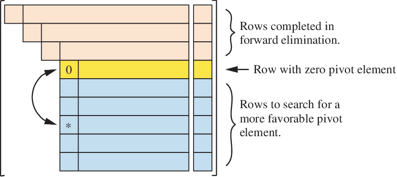
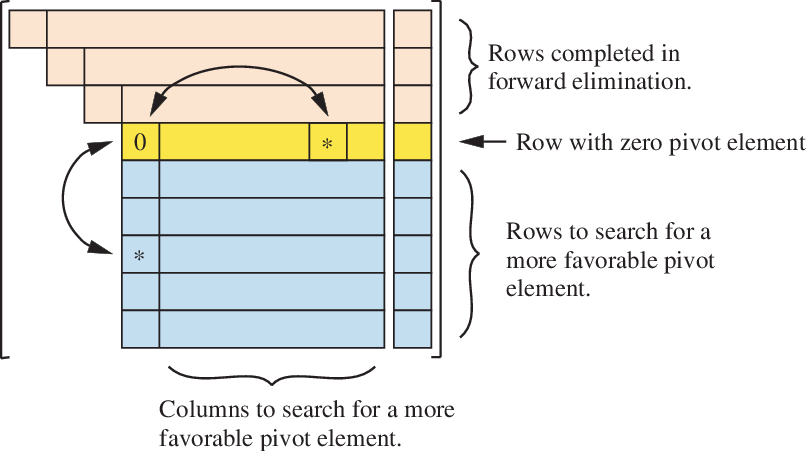
1) First choose \(i\) so that row \(i\) in \({\bf A}\) has the largest absolute first entry. That is, \(\vert A_{i1}\vert \ge \vert A_{j1}\vert\) for all \(j\). Let \({\bf P}_1\) be the permutation matrix that pivots (shifts) row \(i\) to the first row, and leaves all other rows in order. We can explicitly write \({\bf P}_1\) as
\[{\bf P}_1 = \begin{bmatrix} 0_{1(i-1)} & 1 & 0_{1(n-i)} \\ I_{(i-1)(i-1)} & 0 & 0_{(i-1)(n-i)} \\ 0_{(n-i)(i-1)} & 0 & I_{(n-i)(n-i)} \end{bmatrix} = \begin{bmatrix} 0 & \ldots & 0 & 1 & 0 & \ldots & 0 \\ 1 & \ldots & 0 & 0 & 0 & \ldots & 0 \\ \vdots & \ddots & \vdots & \vdots & \vdots & \ldots & 0 \\ 0 & \ldots & 1 & 0 & 0 & \ldots & 0 \\ 0 & \ldots & 0 & 0 & 1 & \ldots & 0 \\ \vdots & \ddots & \vdots & \vdots & \vdots & \ldots & 0 \\ 0 & \ldots & 0 & 0 & 0 & \ldots & 1 \end{bmatrix}.\]2) Write \(\bar{ {\bf A} }\) to denote the pivoted \({\bf A}\) matrix, so \(\bar{ {\bf A} } = {\bf P}_1 {\bf A}\).
3) Let \({\bf P}_2\) be a permutation matrix that leaves the first row where it is, but permutes all other rows. We can write \({\bf P}_2\) as \({\bf P}_2 = \begin{bmatrix} 1 & \boldsymbol{0} \\ \boldsymbol{0} & P_{22} \end{bmatrix},\) where \({\bf P}_{22}\) is an \((n-1) \times (n-1)\) permutation matrix.
4) Factorize the (unknown) full permutation matrix \({\bf P}\) as the product of \({\bf P}_2\) and \({\bf P}_1\), so \({\bf P} = {\bf P}_2 {\bf P}_1\). This means that \({\bf P} A = {\bf P}_2 {\bf P}_1 A = {\bf P}_2 \bar{ {\bf A} }\), which first shifts row \(i\) of \({\bf A}\) to the top, and then permutes the remaining rows. This is a completely general permutation matrix \({\bf P}\), but this factorization is key to enabling a recursive algorithm.
5) Using the factorization \({\bf P} = {\bf P}_2 {\bf P}_1\), now write the LUP factorization in block form as
\[\begin{aligned} %%%%%%%%%%%%%%%%%%%%%%%%%%%%%%%%%%%%%%%%%%%%%%%%%%%%%%%%%%%%%%%%%%%%%% {\bf P A} &= {\bf L U} \\ %%%%%%%%%%%%%%%%%%%%%%%%%%%%%%%%%%%%%%%%%%%%%%%%%%%%%%%%%%%%%%%%%%%%%% {\bf P_2} \bar{ {\bf A} } &= {\bf L U} \\ %%%%%%%%%%%%%%%%%%%%%%%%%%%%%%%%%%%%%%%%%%%%%%%%%%%%%%%%%%%%%%%%%%%%%% \begin{bmatrix} 1 & \boldsymbol{0} \\ \boldsymbol{0} & {\bf P}_{22} \end{bmatrix} \begin{bmatrix} \bar{a}_{11} & \bar{\boldsymbol{a}}_{12} \\ \bar{\boldsymbol{a}}_{21} & \bar{ {\bf A} }_{22} \end{bmatrix} &= \begin{bmatrix} 1 & \boldsymbol{0} \\ \boldsymbol{\ell}_{21} & {\bf L}_{22} \end{bmatrix} \begin{bmatrix} u_{11} & \boldsymbol{u}_{12} \\ \boldsymbol{0} & {\bf U}_{22} \end{bmatrix} \\ %%%%%%%%%%%%%%%%%%%%%%%%%%%%%%%%%%%%%%%%%%%%%%%%%%%%%%%%%%%%%%%%%%%%%% \begin{bmatrix} \bar{a}_{11} & \bar{\boldsymbol{a}}_{12} \\ {\bf P}_{22} \bar{\boldsymbol{a}}_{21} & {\bf P}_{22} \bar{ {\bf A} }_{22} \end{bmatrix} &= \begin{bmatrix} u_{11} & \boldsymbol{u}_{12} \\ u_{11} \boldsymbol{\ell}_{21} & (\boldsymbol{\ell}_{21} \boldsymbol{u}_{12} + {\bf L}_{22} {\bf U}_{22}) \end{bmatrix} %%%%%%%%%%%%%%%%%%%%%%%%%%%%%%%%%%%%%%%%%%%%%%%%%%%%%%%%%%%%%%%%%%%%%% \end{aligned}\]6) Equating the entries in the above matrices gives the equations
\[\begin{aligned} \bar{a}_{11} &= u_{11} \\ \bar{\boldsymbol{a}}_{12} &= \boldsymbol{u}_{12} \\ {\bf P}_{22} \bar{\boldsymbol{a}}_{21} &= u_{11} \boldsymbol{\ell}_{21} \\ {\bf P}_{22} \bar{A}_{22} &= \boldsymbol{\ell}_{21} \boldsymbol{u}_{12} + {\bf L}_{22} {\bf U}_{22}. \end{aligned}\]7) Substituting the first three equations above into the last one and rearranging gives
\[{\bf P}_{22} \underbrace{\Bigl(\bar{A}_{22} - \bar{\boldsymbol{a}}_{21} (\bar{a}_{11})^{-1} \bar{\boldsymbol{a}}_{12}\Bigr)}_{\text{Schur complement } {\bf S}_{22}} = {\bf L}_{22} {\bf U}_{22}.\]8) Recurse to find the LUP decomposition of \(S_{22}\), resulting in \({\bf L}_{22}\), \({\bf U}_{22}\), and \({\bf P}_{22}\) that satisfy the above equation.
9) Solve for the first rows and columns of \({\bf L}\) and \({\bf U}\) with the above equations to give
\[\begin{aligned} u_{11} &= \bar{a}_{11} \\ \boldsymbol{u}_{12} &= \bar{\boldsymbol{a}}_{12} \\ \boldsymbol{\ell}_{21} &= \frac{1}{\bar{a}_{11}} {\bf P}_{22} \bar{\boldsymbol{a}}_{21}. \end{aligned}\]10) Finally, reconstruct the full matrices \({\bf L}\), \({\bf U}\), and \({\bf P}\) from the component parts.
In code the recursive leading-row-column LUP algorithm for finding the LU decomposition of \({\bf A}\) with partial pivoting is:
import numpy as np
def lup_decomp(A):
    """(L, U, P) = lup_decomp(A) is the LUP decomposition P A = L U
       A is any matrix
       L will be a lower-triangular matrix with 1 on the diagonal, the same shape as A
       U will be an upper-triangular matrix, the same shape as A
       U will be a permutation matrix, the same shape as A
    """
    n = A.shape[0]
    if n == 1:
        L = np.array([[1]])
        U = A.copy()
        P = np.array([[1]])
        return (L, U, P)

    i = np.argmax(A[:,0])
    A_bar = np.vstack([A[i,:], A[:i,:], A[(i+1):,:]])

    A_bar11 = A_bar[0,0]
    A_bar12 = A_bar[0,1:]
    A_bar21 = A_bar[1:,0]
    A_bar22 = A_bar[1:,1:]

    S22 = A_bar22 - np.dot(A_bar21, A_bar12) / A_bar11

    (L22, U22, P22) = lup_decomp(S22)

    L11 = 1
    U11 = A_bar11

    L12 = np.zeros(n-1)
    U12 = A_bar12.copy()

    L21 = np.dot(P22, A_bar21) / A_bar11
    U21 = np.zeros(n-1)

    L = np.block([[L11, L12], [L21, L22]])
    U = np.block([[U11, U12], [U21, U22]])
    P = np.block([
        [np.zeros((1, i-1)), 1,                  np.zeros((1, n-i))],
        [P22[:,:(i-1)],      np.zeros((n-1, 1)), P22[:,i:]]
    ])
    return (L, U, P)
The properties of the recursive leading-row-column LUP decomposition algorithm are:
-
The computational complexity (number of operations) of the algorithm is \(\mathcal{O}(n^3)\) as \(n \to \infty\).
-
The last step in the code that computes \({\bf P}\) does not do so by constructing and multiplying \({\bf P}_2\) and \({\bf P}_1\). This is because this would be an \(\mathcal{O}(n^3)\) step, making the whole algorithm \(\mathcal{O}(n^4)\). Instead we take advantage of the special structure of \({\bf P}_2\) and \({\bf P}_1\) to compute \({\bf P}\) with \(\mathcal{O}(n^2)\) work.
Solving linear systems using LUP decomposition
Just as with the plain LU decomposition, we can use LUP decomposition to solve the linear system \({\bf A x }= {\bf b}\). This is the linear solver using LUP decomposition algorithm.
The properties of this algorithm are:
- The algorithm may fail. In particular if \({\bf A}\) is singular (or singular in finite precision), U will have a zero on it’s diagonal.
- The number of operations in the algorithm is \(\mathcal{O}(n^3)\) as \(n \to \infty\).
The code for the linear solver using LUP decomposition is:
import numpy as np
def linear_solve(A, b):
    """x = linear_solve(A, b) is the solution to A x = b (computed with partial pivoting)
       A is any matrix
       b is a vector of the same leading dimension as A
       x will be a vector of the same leading dimension as A
    """
    (L, U, P) = lup_decomp(A)
    x = lup_solve(L, U, P, b)
    return x
Example: matrix for which LUP decomposition succeeds but LU decomposition fails
Recall our example of a matrix which has no LU decomposition:
\[{\bf A} = \begin{bmatrix} 0 & 1 \\ 2 & 1 \end{bmatrix}.\]To find the LUP decomposition of \({\bf A}\), we first write the permutation matrix \({\bf P}\) that shifts the second row to the top, so that the top-left entry has the largest possible magnitude. This gives
\[\overbrace{\begin{bmatrix} 0 & 1 \\ 1 & 0 \end{bmatrix}}^{P} \overbrace{\begin{bmatrix} 0 & 1 \\ 2 & 1 \end{bmatrix}}^{A} = \overbrace{\begin{bmatrix} 2 & 1 \\ 0 & 1 \end{bmatrix}}^{\bar{A}} = \overbrace{\begin{bmatrix} 1 & 0 \\ 0 & 1 \end{bmatrix}}^{L} \overbrace{\begin{bmatrix} 2 & 1 \\ 0 & 1 \end{bmatrix}}^{U}.\]Review Questions
- Given a factorization \({\bf P A} = {\bf LU}\), how would you solve the system \({\bf A}\mathbf{x} = \mathbf{b}\)?
- Understand the process of solving a triangular system. Solve an example triangular system.
- Recognize and understand Python code implementing forward substitution, back substitution, and LU factorization.
- When does an LU factorization exist?
- When does an LUP factorization exist?
- What special properties do \({\bf P}\), \({\bf L}\), and \({\bf U}\) have?
- Can we find an LUP factorization of a singular matrix?
- What happens if we try to solve a system \({\bf A}\mathbf{x} = \mathbf{b}\) with a singular matrix \({\bf A}\)?
- Compute the LU factorization of a small matrix by hand.
- Why do we use pivoting when solving linear systems?
- How do we choose a pivot element?
- What effect does a given permutation matrix have when multiplied by another matrix?
- What is the cost of matrix-matrix multiplication?
- What is the cost of computing an LU or LUP factorization?
- What is the cost of forward or back substitution?
- What is the cost of solving \({\bf A}\mathbf{x} = \mathbf{b}\) for a general matrix?
- What is the cost of solving \({\bf A}\mathbf{x} = \mathbf{b}\) for a triangular matrix?
- What is the cost of solving \({\bf A}\mathbf{x} = \mathbf{b}_i\) with the same matrix \({\bf A}\) and several right-hand side vectors \(\mathbf{b}_i\)?
- Given a process that takes time \(\mathcal{O}(n^k)\), what happens to the runtime if we double the input size (i.e. double \(n\))? What if we triple the input size?
ChangeLog
- 2018-02-28 Erin Carrier ecarrie2@illinois.edu: fix error in ludecomp() code
- 2018-02-22 Erin Carrier ecarrie2@illinois.edu: update properties for solving using LUP
- 2018-01-14 Erin Carrier ecarrie2@illinois.edu: removes demo links
- 2017-11-02 John Doherty jjdoher2@illinois.edu: fixed typo in back substitution
- 2017-11-02 Arun Lakshmanan lakshma2@illinois.edu: minor fix in lup_solve(), add changelog
- 2017-10-25 Nathan Bowman nlbowma2@illinois.edu: added review questions
- 2017-10-23 Erin Carrier ecarrie2@illinois.edu: fix links
- 2017-10-20 Matthew West mwest@illinois.edu: minor fix in back_sub()
- 2017-10-19 Nathan Bowman nlbowma2@illinois.edu: minor existence of LUP
- 2017-10-17 Luke Olson lukeo@illinois.edu: update links
- 2017-10-17 Erin Carrier ecarrie2@illinois.edu: fixes
- 2017-10-16 Matthew West mwest@illinois.edu: first complete draft