Simulating an Ising Model#

In this page, you will write Monte Carlo code to sample configurations from the Ising model with the correct probability.

Minimal background#

The Ising model#

The Ising model is one of the drosophila of physics. At first look, it’s a simple model of crystalline materials which attributes magnetism to the orientation of magnetic moments on a lattice, summarized by the Hamiltonian or energy

\[ E = - \sum_{i,j} J_{ij} s_i s_j + \sum_i h_i s_i. \]

The variables $s_i$ express the possible orientations for each moment, while the entries $J_{ij}$ of the (symmetric) interaction matrix characterize the interaction energy of moments $i$ and $j$. The value $h_i$ specifies a magnetic field on each site $i$.

Ising’s original formulation (often referred to as the Ising model) considers moments with two orientations, $s_{i} = \pm 1$, which only interact with their nearest neighbors. Below we will call this the two-dimensional Ising model.

A configuration of an Ising model is a specification of every moment’s orientation — an assignment of values to the $s_i$ variable for all moments in the system. For our purposes, configurations are ‘snapshots’ of the system which our simulator will hold in memory, like a vector containing $\pm 1$ in its $i$th entry to specify whether moment $i$ points up or down.

Statistical Mechanics#

There are a couple facts we need to know about statistical mechanics.

(1) We can specify configurations of our system $c.$ In the case of an Ising model, the configuration is the orientation of each spin.

(2) Each configuration $c$ has an energy $E(c)$. We’ve already seen this for the Ising model.

(3) For classical systems in contact with an energy reservoir of temperature $T$, the probability $P$ of finding the system in configuration $c$ is

$P(c) = \frac{e^{-\beta E(c)}}{\sum_c e^{-\beta E(c)}}$

where $E(c)$ is the configuration’s energy and $\beta \equiv 1/(kT)$ with $k$ Boltzmann’s constant and $T$ is the temperature. We will work in units where $k=1.$

Markov Chains#

We have just learned that statistical mechanics tells us that if we look at the system, each configuration $c$ appears with probability $P(c)\sim \exp(-\beta E(c))$. Our first goal is to implement an algorithm which gives us configurations $c$ with probability $P(c)$.

One such algorithm is markov chain Monte Carlo.

A Markov chain is a process where you are at some state $c$ (i.e. a configuration) and then you choose another state $c'$ with a probability that only depends on $c$. In other words, you can’t use the fact that previously you were at configuration $b$ to decide the probability $P(c \rightarrow c')$ you’re going to go from $c$ to $c'$. This process is called a memoryless process.

As long as you do a (non-pathalogical) random walk in a memoryless way, you’re guaranteed that, after walking around enough, that the probability you are in configuration $c$ is some $\pi(c)$. $\pi$ is called the stationary distribution. Different markov chains will have different stationary distributions. A Markov chain is non-pathological if:

It is aperiodic; it doesn’t cycle between configurations in a subset of the system’s full configuration space.
It is connected; given two configurations, there is a path with non-zero probability that the chain could (but not necessarily will) follow to get from one to the other.

To simulate the Ising model, we wish to build a markov chain which has the stationary distribution $\pi(c) \sim \exp(-\beta E_c)$. We will do so with a very famous algorithm which lets us build a Markov chain for any $\pi(c)$ we want.

The Metropolis-Hastings algorithm#

If you know your desired stationary distribution, the Metropolis-Hastings algorithm provides a canonical way to generate a Markov chain that produces it. The fact that you can do this is amazing! The steps of the algorithm are:

Start with some configuration $c$
Propose a move to a new trial configuration $c'$ with a transition probability $T(c\rightarrow c')$
Accept the move to $c'$ with probability $\min \left(1, \frac{\pi(c')}{\pi(c)}\frac{T(c'\rightarrow c)}{T(c \rightarrow c')} \right)$

The first step is straightforward, but the latter two deserve some explanation.

How $T(c\rightarrow c')$ is picked: Choosing a procedure for movement between configurations is the art of MCMC, as there are many options with different strengths and weaknesses. In the simplest implementations of the Metropolis algorithm we choose a movement procedure where forward and reverse moves are equiprobable, $T(c \rightarrow c') = T(c' \rightarrow c)$.

Question to think about: How do equiprobable forward and reverse moves simplify the Metropolis algorithm?

Acceptance condition: To construct a Markov chain which asymptotes to the desired distribution $\pi$, the algorithm must somehow incorporate $\pi$ in its walk through configuration space. Metropolis does this through the acceptance ratio

\[ \alpha \equiv \frac{\pi(c')}{\pi(c)}\frac{T(c'\rightarrow c)}{T(c \rightarrow c')}. \]

Notice how the first factor in $\alpha$ is the relative probability of the configurations $c'$ and $c$. Assuming that $T(c \rightarrow c')=T(c' \rightarrow c)$, we have that $\alpha > 1$ indicates that $c'$ is more likely than $c$, and the proposed move is automatically accepted. When $\alpha < 1$, $c'$ is less probable than $c$, and the proposed move is accepted with probability $\alpha$.

Question to think about: Why are moves with $\alpha < 1$ accepted with probability $\alpha$, rather than outright rejected?

States and parameters#

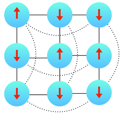
For our simulation, we are going to work on a two-dimensional lattice, have no magnetic field ($h_i=0$) and set $J_{ij}=J$ for all $i$ and $j$ being nearest neighbors (and zero otherwise). This leaves us with an energy

\[E = -J \sum_{(x,y)} s_{(x,y)} s_{(x+a,y+b)}\]

where $(a,b) \in \{(1,0) , (0,1), (-1,0), (0,-1)\}$

For this project we will be working on a $L \times L$ grid (where $L$ is 3 or 27 or 81).

We are going to represent the state of our spins by a $L \times L$ array which can have either a -1 (spin-down) or 1 (spin-up). To set up a random initial conidition you can do np.random.choice([1,-1], (L,L)) in python. In C++, there are two approaches to storing the two dimensional array. One approach is to use the STL: vector<vector<int> > spins. Another option is to use Eigen (see here) where you will use MatrixXi.

This approach will work for square grids (and is what you want to do for this project!). In some cases, you want a more complicated lattice (triangular, pyrochlore) and have different parameters for $J_{ij}$ and $h_i$. In that case, instead of storing it as a grid you can alternatively store it as a graph. This below is just for your edification for future uses.

Storing your configuration as a graph.

A more general way to store your configuration is to put your spins (and magnetic field) on nodes of a graph and the coupling constants $J_{ij}$ as edges.

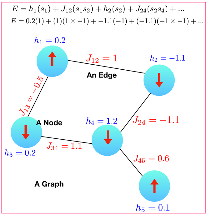
A graph has a bunch of nodes (each node $i$ has a state $s_i$ which is either spin-up or spin-down and has a magnetic field $h_i$) and a bunch of edges (each edge has a $J_{ij}$ on it). Then, if you want a grid you can just choose a graph that is grid-like.

Now there are two questions: how do you represent this inside your code and how do you get the code to know about the graph that you want.

Representing your spins: Here is what I did in my code. I wrote an Ising class which has two vectors which represent the state of the nodes and their magnetic fields (i.e. vector<int> spins and vector<double> h). Then, I stored a neighbor vector. The i’th element in the neighbor vector stores a list (or vector) of neighbors with their respective coupling constants. In other words, for the graph above, you want to be storing the following inside your computer:

Node: (neighbor, J)  (neighbor, J) (neighbor, J) ...
(2, 1)  (3,-0.5)
(1,1)  (4,-1.1)
(1,-0.5) (4,1.1)
(2,-1.1) (3,1.1) (5,0.6)
(4,0.6)

I stored this as vector<vector<pair<int, double> > > neighbors where the pair<int,double> stores the node you are a neighbor to and the weight.

Setting up your graph: Setting up your Ising model this way gives you a lot of flexibility. But now you need some way to tell your code what particular graph you want (maybe the one above or a grid, etc).

I recommend doing this by reading two files. A “spins.txt” which tells you the value of $h_i$ for spin $i$ and a “bonds.txt” which tells you which spins are connected and what their coupling constants are.

For the first graph above: bonds.txt

2 1.0
3 -0.5
4 1.1
4 -1.1
5 0.6

spin.txt

0.2
-1.1
0.2
1.2
0.1

Then just write some sort of Init() function for your Ising model to read in the graph. Also, go ahead and write yourself a python code that generates the relevant graph for a two-dimensional Ising model on a square grid. Now, any time you want to run a different Ising model, you just have to change these files.

Computing the Energy#

The next step in putting together your Ising model is learning how to compute the energy $E(c)$ of a configuration. Write some code (i.e def Energy(spins)) which allows you to do this.

In addition to computing the energy for a single configuration, it’s going to be critical to be able to compute the energy difference between two configurations that differ by a single spin flip (i.e. def deltaE(spin_to_flip))

Why is this? Because the acceptance criterion we are going to use is the ratio of $\exp[-\beta E_\textrm{new}]/\exp[-\beta E_\textrm{old}]=\exp[-\beta \Delta E]$.

Go ahead and make this function. Make sure that the function takes time $O(1)$ and not time $O(N)$ (i.e. don’t call Energy(spins) twice).

Comment about computational complexity: One of the themes of this class is to think about the scaling of your algorithms (like we did thinking about various options for quantum computing). Let’s do this for computing an energy difference. One thing you can do is compute the energy, flip the spin, compute the energy, and subtract. How long does this take? It takes $O(N + B)$ time where $N$ is the number of spins and $B$ is the number of bonds. Find a way to do it with a time that is proportional to $O(1)$.

At this point you should be able to store a configuration of spins and compute energy and energy differences on them.

Testing

Set up a $3 \times 3$ grid and compute the energy of some spin configuration both by hand and with your code to make sure it’s the same
Compute the energy difference of flipping a single spin both by
- using your Energy() function before and after a spin flip.
- using your deltaE() function.

Both approaches for computing the energy should be the same. Another reasonable test is to compute the energy of a number of configurations that you can evaluate by hand (all spin-up, etc) and verify that it works.

Writing MCMC#

We now want to put together the Monte Carlo. The basic operation, which we call a step is to do the following (many times):

Choose a new configuration $c'$ with some probability $p(c \rightarrow c')$ given the current configuration $c$. The simplest method is to choose a random spin and flip it. In this case both $T(c \rightarrow c') = T(c' \rightarrow c) = 1/N$ (where $N$ is the number of spins). Therefore the ratio of $T$ cancel in the acceptance probability $\alpha$).
Evaluate the difference in energy $\Delta(c,c) \equiv E(c') - E(c)$
If $\frac{T(c' \rightarrow c)}{T(c \rightarrow c')} \exp[-\beta \Delta(c,c')]>\textrm{ran}(0,1)$ then accept the new configuration $c'$. Otherwise leave the old configuration $c$

We will call a sweep doing $N$ steps.

You will typically need to do a certain number (maybe 20) sweeps before you should start collecting data. This is called the equilibration time and is required because you need the Markov Chain to forget about your initial condition.

Then you can take a measurement every sweep. There is no need to measure more often then this (and doing so will just slow down the simulation).

This is going to look something like this (in c++)

for (int sweep=0;sweep<10000;sweep++){
    for (int i=0;i<N;i++){
        //Pick a random spin and try to flip it
    }
    //measure your histogram or energy, etc. 
}

or (in python)

for sweep in range(0,10000):
    for step in range(0,N):
        #flip spins
    # measure 

Grading

For your $3 \times 3$ grid, run your Monte Carlo and make a histogram of the configurations. To do this, you should take a snapshot of your spin-configuration every sweep. Your spin-configuration can be flattened down to nine spins (i.e. $\uparrow, \downarrow, \uparrow ... \uparrow)$. This can be turned into a nine-bit binary number ($101..1$) which can then be turned into an integer from 0 to $2^9-1.$ You then have an integer for every sweep from which to make a histogram.

Then, compare this histogram against the theoretical values - i.e you can compute the energy of all $2^9$ configurations (using python) and then you can use the formula $\exp[-\beta E(c)]/Z$ (where $Z$ is the normalization) to make the theory graph from this.

You should have both graphs on top of each other on the same plot (maybe one with points and one with lines) to see that they agree. There is going to be some error bar on your Monte Carlo data so they don’t have to match exactly.

Note, that this is a great way to test your code. It’s only going to work with a small number (i.e. 9) of spins. If you tried to do this with 25 spins, you would need much too large a histogram.

How often should you take snapshots (or more generically compute observables)

The promise of MCMC is that after a “long enough time” $T$, you should get a random sample (we unfortunately don’t know $T$ a-priori - it’s at least one sweep but could be many sweeps). Roughly you want to measure an observable or add to your histogram every $T$ sweeps.

Q: What happens if you take snapshots too infrequently? You end up just wasting some time. The samples are still independent.

Q: What happens if you take snapshots too frequently? That’s a little more subtle. If you take snapshots too soon then you are in trouble. This means that you should wait a fair amount of time before you start measuring snapshots.

If you wait enough time for the first snapshot and then take measurements more frequently then you are still ok. It’s just you have to be careful with your errorbars because subsequent snapshots may be correlated.

Later on we will see how to estimate $T$. For this simulation,let’s just assume that $T$ is about a sweep. Wait 10 sweeps before you begin measuring snapshots. Then take a snapshot every sweep. Error bars for your histogram: If you have $k$ samples in a bin then your error should be $\sqrt{k}$.

If you are using C++, your code will be very efficient (although make sure you are compiling with -O3 or it will be much too slow!)

In python unfortunately, this will turn out to be very slow especially if you are using for loops.

The code will be correct but it will take a very long time (this doesn’t matter and won’t necessarily show up for the $3 \times 3$ system but will mean you have to wait a long time for the larger systems you will do later in this assignment).

Speeding Up Your Code (especially python)#

Extra Credit (5 points)

There is 5 points to get your code working quickly. You can earn this by having your code do 1000 sweeps of an $81 \times 81$ lattice in less then 15 seconds. If you’re using C++ (which is harder then python) this will be easy. If you’re using python, see a description below for how to accomplish this.

To speed up your python code, what you want to do is avoid having a for-loop over steps; instead you should work with many of the spins at once.

Heat Bath#

Before we do this, though, we need to make a minor change to the Monte Carlo move we are making (otherwise we accidentally get a pathological Markov Chain)

Our current move is

pick a random spin
consider flipping it

We are going to switch to another move - the heat bath move.

Pick a random spin (say spin $i$)
Consider
- making it spin-up with probability $\frac{\exp[-\beta E(...\uparrow_i,...)]}{\exp[-\beta E(...\uparrow_i,...)]+\exp[-\beta E(...\downarrow_i,...)}$
- making it spin-down with probability $\frac{\exp[-\beta E(...\downarrow_i,...)]}{\exp[-\beta E(...\uparrow_i,...)]+\exp[-\beta E(...\downarrow_i,...)}$

Notice that this move doesn’t actually care what the current spin was! This means sometimes you are going to replace a configuration with the same configuration. (If you think for a minute you can convince yourself that if you’re considering doing this, you accept it with probability one).

When we do this we need to be a little careful with the acceptance probability. When we were flipping a spin, $T(c\rightarrow c') = T(c' \rightarrow c) =1/N$ and the ratio of the $\frac{T(c' \rightarrow c)}{T(c \rightarrow c')}=1$. Therefore it didn’t come into the acceptance probability.

In the new move, let’s assume we are moving from

our current configuration $c = \{...\downarrow_i...\}$ to
our new configuration $c' = \{...\uparrow_i...\}$

Then we find that

$T(c \rightarrow c')=(1/N) \frac{\exp[-\beta E(...\uparrow_i,...)]}{\exp[-\beta E(...\uparrow_i,...)]+\exp[-\beta E(...\downarrow_i,...)}$ (since this is the probability of choosing spin-up) and
$T(c' \rightarrow c)=(1/N) \frac{\exp[-\beta E(...\downarrow_i,...)]}{\exp[-\beta E(...\uparrow_i,...)]+\exp[-\beta E(...\downarrow_i,...)}$.

Therefore, the ratio

\[\frac{T(c' \rightarrow c)}{T(c \rightarrow c')} = \frac{\exp[-\beta E(...\downarrow_i,...)]}{\exp[-\beta E(...\uparrow_i,...)]}\]

But our ratio of Boltzmann factors gives us $$\frac{\pi(c')}{\pi(c)} = \frac{\pi(\{...\uparrow_i...\})}{\pi(\{...\downarrow_i...\})} = \frac{\exp[-\beta E(...\uparrow_i,...)]}{\exp[-\beta E(...\downarrow_i,...)]}$$

Therefore the total acceptance ratio (the product of these two terms)

\[\frac{T(c' \rightarrow c)}{T(c \rightarrow c')} \frac{\pi(c')}{\pi(c)} =1 \]

Therefore, we accept 100% of the moves that we consider (although this isn’t as good as it sounds because some of that time we are accepting a move that doesn’t do anything).

If you do a little bit of algebra, you can rewrite this entire move so that the probability you flip your spin (i.e. the probability you compare to a random number) is $(1+1/\exp(-\beta \Delta E))^{-1}$ where $\Delta E$ is the energy difference between your current configuration and the one with the spin-flipped. Replace your acceptance criterion with this new criterion. This should be the only change you need. Verify you get the same answers.

Many Spins At Once#

Let’s consider the $7 \times 7$ lattice. Which spins can we flip simultaneously?

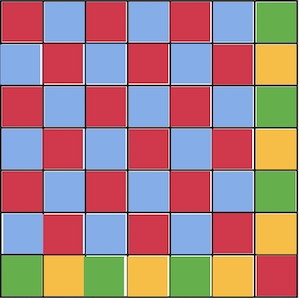
We can consider flipping all of the red squares at once, because the red squares aren’t neighbors of any other red squares (even with the periodic boundary conditions) and so if we flip them all at one time, there isn’t going to be any conflicts. The same is true of the blue, yellow, and green colors (the yellow and green exist to deal with the boundary conditions and the odd-size lattice).

In python, we can access all the colors by doing

# This is for a L x L lattice
x,y=np.indices((L,L))
red=np.logical_and((x+y) % 2==0   , np.logical_and(x<L-1,y<L-1))
red[L-1,L-1]=True
blue=np.logical_and((x+y) % 2==1   , np.logical_and(x<L-1,y<L-1))
green=np.logical_and((x+y) % 2==0   , np.logical_or(x==L-1,y==L-1))
green[L-1,L-1]=False
yellow=np.logical_and((x+y) % 2==1   , np.logical_or(x==L-1,y==L-1))

For each color (say red as an example)

write a function that computes the $\Delta E$ for all the red spins without using any for-loops. Two things you might find useful here are that spins[red] will access all the red spins. In addition, np.roll(spins,1,axis=0) will return an array where all the spins are rolled over to the right.
After calling this function, write one line of python that returns an array which says which red spins should be flipped.
Write one line of python which flips just those spins.

Just to give a sense, this is how long my version of the naive python code and the efficient python code take for 1000 sweeps:

Slow Code Wall time: 1min 20s
Efficient Code Wall time: 1.06 s

Even Faster Code#

At this point the primary bottleneck of your code is that the Markov chain has a large autocrrelation time near the critical point. This phenomena is called critical slowing down.

Extra Credit (1 point)

Plot the autocorrelation time of your simulation as a function of $\beta$. You should see that it explodes at the critical point.

To help resolve this problem, essentially you have to move to more sophisticated Monte Carlo techiques. The most general of these is parallel tempering.

For this particular model, though, you have a lot of other choices. The most famous of these choices is the Wolff algorithm. The Wolff algorithm is a cluster-move which flips an entire cluster instead of a single spin at a time.

Another alternative is the worm algorithm. The worm algorithm rewrites the Ising model using a totally different set of variables.

Extra Credit (5 point)

Implement the Wolff algorthim and worm algorithm and measure the autocorrelation times as a function of $\beta$ showing that they both do better then the single-spin flip techniques.

Coupling From the Past#

Extension and Extra Credit (10 points)

By writing a Markov Chain Monte Carlo, you’ve produced a code which samples from the Boltzmann distribution for an Ising model - at least if we look away for long enough. Unfortunately, we don’t know how long that necessarily needs to be. In practice, this is rarely a problem. Nonetheless, it would be satisfying if there was an algorithm that exactly sampled from the Boltzmann distribution of the Ising model with no heurestics or additional approximations. There is such an algorithm: coupling from the past. This algorithm is on my list of 10 algorithms I didn’t believe could accomplish what it was claiming when I first heard it (automatic differentiation is also on that list).

Computing in Physics (Phy446)

Simulating an Ising Model

Contents