The Renormalization Group

Note: On this page we are going to interchangably use $\beta J$, $J$ and $\beta$. This is because it’s equivalent to think that $\beta$ is constant and we change $J$ or visa versa because the only place where either variable shows up is in the formula $\exp [-\beta J]$ and they both show up together.

References

• Ken Wilson’s 1979 Scientific American article on renormalization, “Problems in Physics with Many Scales of Length”. (Possible direct pdf link)

Minimal background

The Ising model was immortalized in physics history not by Ising, but by researchers who followed. In his original work (his PhD thesis, 1924), Ising considered only one-dimensional magnets and famously found that his namesake model did not describe a phase transition between paramagnetism and ferromagnetism, despite belief that it should. Interest in the model waned until 1936, when Rudolf Peierls argued that two-dimensional variants of the model do exhibit ferromagnetic phase transitions. In 1944, nearly a decade after Peierls’ argument, Lars Onsager published an exact solution of the two-dimensional model — so crafty that its details still vex most physicists — validating Peierls’ conclusions. Turns out the Ising model is a good model of ferromagnetism, but dimensionality matters.

Evidently reliance on exact solutions is a poor method for identifying the interesting phases of models; we’d like to unpack more physics than two dimensions worth from a promising model over 20 years. It’s for this reason that Ken Wilson’s formulation of the renormalization group — following pioneering work by Gell-Mann and Low, Kadanoff, and undoubtedly many others — is held in such high regard.

The renormalization group (RG) is a theory of theories. Roughly speaking, it’s a general method to determine how the physics of a particular model, expressed by a Hamiltonian $H$ involving a set of coupling constants $\{J_i\}$, depends on dimensionality and (principally) scale. More concretely, it’s a dynamical theory of the space of Hamiltonians. To make sense of RG we must step back and think broadly about how we write down physical models.

Abstractly, we can imagine models as living in some infinite-dimensional space where the axes represent every conceivable interaction of the model’s microscropic constituents. For magnetism models, one axis might be interaction with an external magnetic field, $\mu B\sum _i{s}_i$, another nearest-neighbor interactions, $J_1\sum _{⟨ij⟩}{s}_i{s}_j$, another next-nearest neighbor interactions, $J_2\sum _{\text{n.n.n.}}{s}_i{s}_j$, many more for all four-moment interactions, $\sum _{ijkl}{K}_{ijkl}{s}_i{s}_j{s}_k{s}_l$, and so on. To identify a concrete model, we merely specify values for the coupling constants $\mu B$, $J_1$, $J_2$, $\{K_{ijkl}\}$, etc., which parameterize the model’s extension along each axis. Thus the plain Ising model lives along the $J_1$ (and sometimes $\mu B$) axis, with all other coupling constants taken as 0.

Outcomes of measurements depend immensely on the scales at which they’re taken, even when studying a single system. (Consider the results you might get measuring: the pressure of a balloon using its entire surface versus a square-angstrom patch; particles produced by 1eV proton collisions versus 10 TeV proton collisions.) Naively modeling, we would write down very different looking Hamiltonians to describe the physics at each scale. If it’s truly possible to attribute one Hamiltonian to the microscopic stuff in a system, there must be some way to determine how that Hamiltonian evolves as the system is probed at different scales.

RG provides such a methodology by establishing differential equations for a model’s coupling constants. Viewing coupling constants as functions of some observation scale (be it energy or length), it determines the significance of interactions as a system is examined at increasing/decreasing scale, showing how the constants grow or shrink.

On this page we’ll walk through a discrete, numerical application of RG to the Ising model. Iteratively transforming the model to larger and larger lattice sizes (lower and lower energies), we’ll find that it describes multiple phases of matter at low energy.

---

Implement the renormalization group with an Ising model simulator

We would now like to use our Ising model simulation to understand something about the renormalization group. RG tells us to approach the model in the following way:

• Take your initial simulation

• Coarse grain it in some way (i.e. perform a scale transformation)

• Interpret the new simulation as looking just like the old simulation, but with different parameters.

In our implementation the parameter we will tune is the nearest-neighbor coupling constant $J$. Our objective is to define a function $R(J)$ which eats $J$ and generates a new constant $J^{\prime }=R(J)$ representing the coupling’s value after coarse graining.

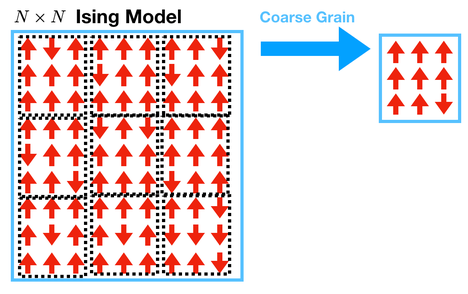
Coarse graining

The first step of renormalization is coarse-graining. To do this, we will take blocks of $3\times 3$ spins and turn them into a single spin by following a rule. The new spin is determined by majority voting: if most of the spins are up, make the coarse-grained spin up; if most of the spins are down, make the coarse-grained spin down.

Grading

Generate snapshots of spin configurations for $\beta J\in [0.0,0.3,0.4,0.5,0.6,\mathrm{\infty }]$ for

• an $81\times 81$ spin configuration

• a single coarse-grained $27\times 27$ spin configuration and

• a double coarse-grained $9\times 9$ configuration.

Can you see where the transition is?

Now we want to do something more quantative. We will take an Ising model on an $N\times N$ lattice, coarse grain it to a $N/3\times N/3$ lattice, then match the properties of the coarse-grained lattice to a natively $N/3\times N/3$ lattice. This will provide a way to generate the function $R$.

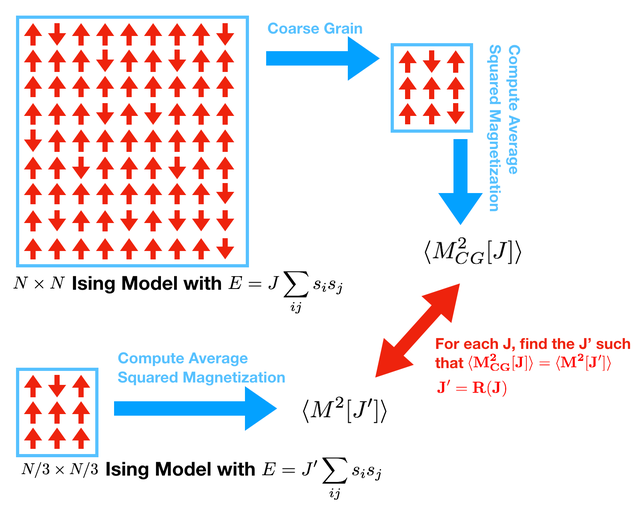
To accomplish this we must find some quantitative feature of the model that can be compared to itself after coarse graining. Concretely, we will match the $⟨M^2⟩$. The approach is the following:

• Run your simulator on an $N\times N$ model with a coupling constant $J$.

  • While this simulator is running, compute the coarse-grained $N/3\times N/3$ model

  • Measure $⟨M_{CG}^2[J]⟩$ of the coarse grained model.

  • Make a graph of this for every $\beta$

• Run your simulator on an $N/3\times N/3$ model.

  • Measure $⟨M^2[J^{\prime }]⟩$ of the coarse grained model.

  • Make a graph for this for every $\beta$

• Now plot your two curves on top of each other.

  • Where the curves intersect are fixed points.

• From these two curves you should be able to generate a graph of $R(J)$ vs. $J$

Testing

The coarse grained calculation is very easy to mess up.

• Look at your coarse-grained snapshots and convince yourself that they look right.

• Figure out how to compute the $\beta =0$ result for the coarse-grained $27\times 27$ lattice for $⟨M^2⟩$ analytically or using five lines of python. Check that this matches what you got in your Monte Carlo. This is an important test and will catch lots of mistakes.

Grading

Plot for your native $27\times 27$ lattice and coarse-grained $27\times 27$ lattice $⟨M^2⟩$ vs $\beta$. You must put on your plot a point for the $\beta =0$ “testing” point for both these curves.

Getting $R(J)$

You should have a coarse-grained and native $27\times 27$ curves. Now you want to produce $R(J)$. Here’s one approach:

• Graph the native curve as $⟨M^2⟩$ vs. $\beta$. You want to interpolate this using scipy.interpolate.interp1d where the interpolation takes $⟨M^2⟩$ and gives back $\beta J$. This is backwards from how you’ve graphed it naively

• Go through the coarse grained curve and find the closest $\beta$ on the native curve for each value of $\beta$ on the coarse-grained curve.

Grading

Put the plot for $R(J)$ vs. $J$ in the document for $0<J<1$. Also draw $y=x$ on this plot. Where are the fixed points of this curve (the values such that R(J)=J)? The fixed points are the places on your plot where the $R(J)$ curve intersects the line $y=x$ (understand why this is). What is the critical transition temperature?

Extension

You’ve now succesfully implemented the RG approach for the 2D Ising model. Congratulations! It is an interesting exercise to try the same approach for the 1D Ising model (where you should find no phase transition) and the 3D Ising model (where you should also be able to compute the critical exponent $\nu$ as described below. Another fun activity is to work on the 2D Ising model but with more parameters (i.e. add in a magnetic field and determine the RG flow as a function of both $\beta$ and $h$.

Extension

In this work, you have performed the RG flow by running simulations at two different system sizes and the matching them. This is conceptually the simplest thing to do. In practice, as the number of coupling constants gets large, though, this would become unwieldy. There is a way to determine the flow with simulations at a single temperature using the Monte Carlo Renormalization Group

Extension

So far we’ve seen how to do the renormalization group using Monte Carlo. There is an alternative performing RG using tensor networks called TNRG that can be used to compute the critical exponent of things like Ising models.

Critical Exponents and Stability of Fixed Points

The whole point of the renormalization group is that you should be able to apply the renormalization procedure over and over again and flow to a fixed point which corresponds to a phase. We’ve already seen this in pictures when you coarse grained twice. Now, we are going to see if we can use your $R(J)$ plot to see the same thing. Suppose you start at $J=0.35$. We can then ask what your new $J$ is after the first coarse graining step - it’s $R(0.35)$. Now, suppose we were to do the renormalization procedure again. Well instead of starting at $0.35$ you would start at $R(0.35)$. A nice way to see this graphically is to draw an arrow from $(0.35,R(0.35))$ to $(R(0.35),R(0.35))$. You can do this using pylab.pyplot.arrow(0.35, R(0.35), R(0.35)-0.35,0). The arrow is now pointing at the new spot on the x-axis you would start. And after you apply the RG step you’ll actually be at $(R(0.35),R(R(0.35)))$. Draw the arrow from $(R(0.35),R(0.35))$ to $(R(0.35),R(R(0.35)))$. Now iterative the RG process a couple more times. Do you see what’s happening?

Do this over again starting at $J=0.5$ and draw your arrows.

What you’ve done is show that there are two stable fixed points that correspond to the phases and one unstable fixed point (you only get back to it if you start exactly there) which corresponds to the critical point.

Grading

Add your $R(J)$ curve with the arrows to your document.

You should find that $R(J)$ is linear around the unstable fixed point. Do you? Unstable fixed-points are characterized by a set of universal critical exponents. Many other systems have the same universal critical exponents, even when they are fundamentally different from magnets! For example, the two-dimensional Lennard Jones fluid - has the same critical exponents.

One particular critical exponent, $\nu$, is defined as

$$b^{1/\nu }=\text{slope}$$

where $b=3$ is the ``scale factor’’ we are coarse-graining by.

You should find your critical exponent.

Grading

Add to your document, your critical exponent $\nu$.

Extension

You’ve computed a critical exponent using the renormalization group! There is an alternative approach to computing critical exponents by just looking directly at your data on $⟨M⟩$, $⟨M^2⟩$ and $⟨E⟩$. Critical exponents essentially tell you how these various quantities scale as the temperature approaches the critical point. Without too much work you can look up the 2D Ising model critical point and try to match them with your data.