Physics 363 Fall 2000: Atomic Scale Simulations
Term Project
Shear Flow of a Simple Liquid in a Confined Space
by
Justin Hooper
Jiwen Liu
Ioannis Tziligakis
Contents
Introduction
Two fundamental problems in fluid mechanics are:
The study of the flow of a fluid confined between two fixed walls. The walls are rough and therefore a thin layer of fluid, stationary with each wall, exists close to each wall. This is called the "Poisseuille flow" problem.
The study of planar "Couette flow" where the fluid is confined between two parallel walls that slide relative to one another at a constant rate. In this project we are studying the second case, namely the problem of Shear flow of a fluid of monatomic molecules confined between rough walls.
Our desire in this project was to study the phenomenon of planar Couette flow through the implementation of a molecular dynamics simulation. While multiple attempts have previously been made to investigate such phenomena, we decided to pursue a different pathway in the hopes of being able to investigate the particular manner in which fluids leave and come to rest when introduced to an imposed planar shear flow.
As such, the goal of our project was to implement a non-equilibrium molecular dynamics simulation utilizing a Lennard-Jones reference fluid and an analytically perturbed atomically smooth wall, with shear implemented by coupling an modified Lennard-Jones potential to the analytically perturbed wall, and using this potential to induce shear on the liquid molecules within the system.
Methodology
In an effort to attempt to implement our system, we visualized
a simulation cell, which would have periodic boundary conditions in both the X
and Y directions, with ![]() , and hard, "textured" walls separated by a distance of
, and hard, "textured" walls separated by a distance of ![]() in the Z direction.
The texture in the walls was imposed by a perturbation function, used to
modify the position of the wall/system interface. To this wall, we attached a modified Lennard-Jones potential with
a 9-4 scaling, as is often used for similar calculations. Thus, the wall potential was:
in the Z direction.
The texture in the walls was imposed by a perturbation function, used to
modify the position of the wall/system interface. To this wall, we attached a modified Lennard-Jones potential with
a 9-4 scaling, as is often used for similar calculations. Thus, the wall potential was:
where ![]() is the atomic
diamater,
is the atomic
diamater, ![]() is the well depth of the wall (relative to that of the atoms
in the system),
is the well depth of the wall (relative to that of the atoms
in the system), ![]() is the displacement from the flat (unperturbed) wall, and
is the displacement from the flat (unperturbed) wall, and ![]() is given by:
is given by:
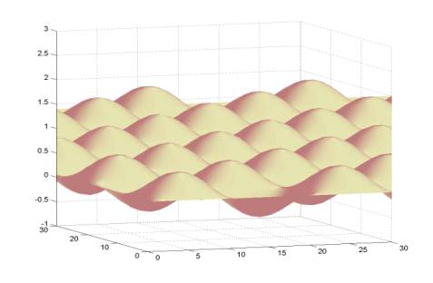
This allows the wall to be "textured" in a periodic and
continuous manner (thus ensuring the that periodic boundary conditions are
maintained in the X and Y directions), while providing a means to shear the
system (through modifying the location of the oscillatory wall force by
advancing the X component of the perturbation by ![]() at each time step. The character of this function is shown
below:
at each time step. The character of this function is shown
below:
The shear force itself is provided by the gradient of the wall potential which, even though the wall potential is taken to be strictly perpendicular to the wall, contains perpendicular potential gradients as well due to the perturbation in the wall surface (as demonstrated below, for a two dimensional system for ease of visualization):
In traditional fashion, the atomic potential for the system was taken to be a standard 12-6 Lennard-Jones potential:
where ![]() is the well depth of the atomic interaction. Together,
is the well depth of the atomic interaction. Together, ![]() and
and ![]() comprise a full basis
set for determination of all system parameters, which can be constructed as
combined quantities of these two fundamental parameters, using only additional
physical constants as necessary.
comprise a full basis
set for determination of all system parameters, which can be constructed as
combined quantities of these two fundamental parameters, using only additional
physical constants as necessary.
Having determined the energetic interactions by which our system would operate, we were left with the decision as to how to advance our system through the integration of the equation of motion. We decided on the Gear predictor-corrector methodology, as it preserves the higher order derivatives of the acceleration (force), which we determined might prove important for our system as it underwent the nonequilibrium motions expected.
The standard Gear predictor algorithm comprises a two step process, the first step of which is to calculate the predicted value of momentum, velocity, acceleration, the first derivative of acceleration, ... based on a Taylor expansion about the value of interest. The second step is to calculate the forces at the predicted point, and form a correction based on the difference between the predicted accelerations and the ones found as a result of the prediction (effectively seeking a position of net zero acceleration, which would indicate a lack of net external forces, and hence an equilibrium position for the particle in question). While it's possible to use any number of time derivatives for the Taylor expansion of the initial predicted quantities, we chose to use a five-value Gear predictor-corrector algorithm, both for it's relatively good speed and relatively decent performance. Additionally, this algorithm is widely available and has been investigated and previously optimized.
Finally, an initial configuration for the system had to be
chosen. For ease of implementation, the
atoms were initially placed within a sub-volume of the box comprised of the
complete X and Y dimensions, and a reduced Z dimension equivalent to the
location of the unperturbed wall plus the maximum wall perturbation magnitude,
plus the magnitude of the molecular diameter of the molecule (mathematically ![]() ). This was done to
insure that the system did not start out in a situation wherein the interaction
of any atom with the perturbed wall was strongly repulsive (or, worse, where an
atom was initialized outside the system).
). This was done to
insure that the system did not start out in a situation wherein the interaction
of any atom with the perturbed wall was strongly repulsive (or, worse, where an
atom was initialized outside the system).
Results
A considerable amount of difficulty was encountered in simply trying to equilibrate the system. With the C code provided, the initial system seemed to contain an excess of potential energy. As such, the system, while initialized at the correct equilibrium kinetic energies, would inevitably, and eventually, begin to undergo wild kinetic energy fluctuations, as shown in this graph:
As a possible explanation for this type of difficulty in coming into equilibrium with the system, it's theorized that a combination of the lack of an available thermostat in the system, coupled with an excessive amount of potential energy in the initialization profile of the system is combining to provide the poor equilibration in the above graph. In a normal, fully periodic system, this would be unlikely, as the system would be allowed to come into equilibrium at whatever temperature is represented by the total energy of the system (kinetic + potential), and then rescaled to the proper system temperature before proceeding. Unfortunately, since our system is bounded by two (theoretically) infinite walls, this type of unbounded kinetic energy poses problems, as the high kinetic energies essentially translate into large velocities for the particles within the system, leading to predictions and or corrections of the particle trajectories which places them far outside the wall of the system, with no deterministic path back into the system.
In order to try to combat this problem, an attempt was made to reflect the particles when they crossed the confining box's boundary. The particle directions were kept in the X and Y directions, but the velocity in the Z direction was directed back into the system interior. Additionally, a "collision" with the wall was considered an act of thermal transfer, and the velocity of the particle was therefore reset to the average requested temperature of the system, in mimicry of a real wall/fluid interaction at which the wall is available to thermally equilibrate the fluid molecules within the system.
While this, by construction, solved the difficulty of the particles moving beyond the system walls, it also tended to inject excess kinetic energy into the system (most likely through placing atoms back into a high potential situation, which they had been trying to escape by moving into the walls in the first place). The above graph shows the consequences of this algorithmic choice, with the areas of large scatter onset corresponding to the original time at which a particle would breach the walls of the system.
It should be stressed that despite the changes in the construction of the system or changes in the control parameters, the same overall characteristic motion of the system remained relatively constant: The system would begin at an average kinetic energy roughly appropriate for the system, then a catastrophic event would transfer kinetic energy from one or more components to the other components, and the system would enter a period of wild instability, inevitably followed by penetration of a particle through the wall (for the unreflected system) or floating point failure as the kinetic energy of the system grew unbounded (for the reflected system).
While dealing with the equilibrium difficulties occupied the majority of our time, we were able to take a brief look at a system to try and determine whether or not we were able to induce a shear velocity profile in the system. The raw velocity data as a function of position within the box is presented below. The left hand wall is undergoing shear, while the right hand wall is held steady. As can be readily seen, the velocity profile is not the expected linear ramping of a velocity from zero to the shear velocity:
While the velocity profile doesn't show the expected shear profile, it is curious that both the overall and kinetic energy of the system rise as the system moves forward through time, exactly as would be expected as if the wall was coupling to the fluid, and thereby imparting energy to the fluid. This energy accumulation is significant, as can be seen here:
As can easily be seen, the energy of the system remains constant for a period, then rapidly diverges, in a manner similar to the difficulties encountered with the equilibration of the system as discussed previously.
Conclusion
Ultimately, the conclusions reached are relatively unrelated to the initial project goals. While our initial goal was to investigate how a system behaved under shear, we ended up discovering (or perhaps reaffirming) that multiple matters of seeming inconsequential nature can play a large role in systematic behavior when running simulations. In this case, our inability to employ traditional methods of thermostat control, coupled with the apparently severe constraints of the two walls enclosing the system led to wildly unexpected behavior. This was even more puzzling once we implemented the particle reflection/temperature renormalization, as it was expected that this would effectively instantaneously remove all the excess heat from a particle, thus rapidly equilibrating the system. It should be noted that, as a quick experiment, upon noticing the fast energy "overload" resulting from reflecting the particles back into the system, the placement of the particles into the system on reflection was randomized in the X and Y direction by multiplying the particle diameter by a normal distribution centered around a zero mean, effectively "jittering" the particle's re-entry into the system volume.
There was a noticeable difference in the rapidity with which the system then approached kinetic energy "overload", allowing, on average, another 3 to 4 times as many iteration steps to proceed before the system failed. While this doesn't directly address the problem of the system, it does provide a bit of a clue into what may be going on within the system. For whatever reason, the system with the wall constraints seems to undergo the following series of phenomena from a generally accepted (crystalline) initial state:
The initial kinetic energy remains relatively constant, with perhaps one or two components (X, Y, Z) exhibiting a slow drift. At some point, the atoms interact, and kinetic energy is transferred from one direction to another. Once kinetic energy is transferred to the Z direction (perpendicular to the walls), a type of "chain" reaction starts, whereby one particle seems to be "bouncing" from one wall to the other. As other particles get near, it imparts its energy to them, and they too begin to exhibit similar behavior. This continues, for an amount of time, until the system breaks down due to particle penetration (with no reflection) or inordinately high kinetic energies (with reflection). We can mitigate these factors to varying degrees, but within the constraints of no externally imposed thermostat, these behaviors persist through reasonable attempts to introduce systematic controls that would be expected to remove such anomalies.
This deviation seems systematic, as can be seen from the energy graphs, which show a similar behavior for the system even when the equilibration problem doesn't factor into the system. This provides yet more evidence that the phenomenon is systematic of the model and/or simulation implementation. While the velocity profile generated shows no clear evidence of shear coupling between the wall and the system, it's unclear whether this is because the system is not coupling to the wall, or if instead any shear effects are relatively minor compared to the magnitude of the average energy of the system.
Future work to investigate this phenomenon should proceed down one of two distinct paths:
Efforts can be made to provide a known initial state in the desired liquid phase (minus any perturbations to a true equilibrium state that would be expected as we go from having a bulk liquid to having a confined liquid). From this initial equilibrium state, it should then be possible to actually investigate the shear characteristics of the fluid, at least for short times. At long times, it's unclear whether the particle reflection/velocity renormalization technique is sufficient to control the shear heating effects, which are expected.
Alternatively, efforts can also be made to quantify the nature and origin of the difficulty of equilibration. The fact that the kinetic energy of the system seems to actually grow over time without shear to increase the energy is disturbing. Determining whether this phenomenon is physical or systematic (due to the integration behavior, force assumptions, or some other combination of factors) would be of interest in this case.
References
While there are a plethora of papers available from a variety of scientific journals about specific systems, our attempts to build this system were carried out from first principle using the information presented in the following two books as a concise reference point for the simulation mechanism.
Allen, M. P. and Tildesley, D. J., Computer Simulation of Liquids, Oxford Science Publications, New York, 1987.
Rapaport, D. C., The Art of Molecular Dynamics Simulation, Cambridge University Press, New York, 1995.
Source Code
This file includes the skeleton of a full simulation of the system described above, including routines (currently untested) to calculate properties of interest such as the velocity autocorrelation function and static structure factor. While the code compiles on the machines tested on, no guarantees are made about whether it will compile on your machine, or if it does whether or not it will produce output of value to you. Most routines are reasonably well commented so that you can see what the code is attempting to do:
Last revised: Dec. 15,2000