Results and Discussion

The optimal structures obtained for different cluster sizes along with their potential energy (in units of $\epsilon$ = 2.17 eV) are shown in fig. 4. All the structures predicted by ECGA agree with those in literature [10] indicating that ECGA was successful in reaching global optimum effectively. Illustrations of a single GA run for the case of 6 and 7 atom clusters are given in figs. 5 and 6 respectively. It can be seen in both cases that in the initial generation the structure is very bad, but ECGA quickly converges to a structure close to the optimal structure and then slightly modifies it to reach the global structure. The energy variation is only in the second or third decimal place in those stages.

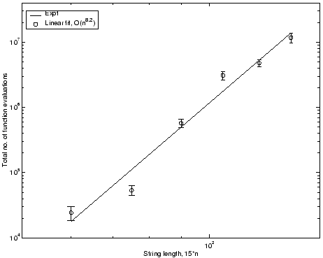
The minimum population size required for different cluster sizes is shown in fig. 7. The minimum population size scales up with the size of the cluster as O(n^4.2). The number of generations taken by ECGA for different cluster sizes is shown in fig. 8. The results show that ECGA converges much faster than those existing in literature, even though the reliability and convergence criteria are much more stringent. This emphasizes the effectiveness of having good operators that preserve good BBs. Finally the number of function evaluations taken by ECGA for different size clusters is shown in fig. 9. The number of function evaluations scales up with the size of the cluster as O(n^8.2). It has to be noted that the high reliability constraint is the reason why the algorithm scales so badly. If fact, if the reliability constraint is reduced to 80%, then the minimum population size scales up as O(n^0.86) and the number of function evaluations scales up as O(n^2.1). As far as we know all the reliability restrictions of all the other existing cluster optimization algorithms are very low (about 10%).

Figure 4: Optimal structures and their total potential energy (in units of $\epsilon$ = 2.17 eV) predicted by ECGA for different cluster sizes.

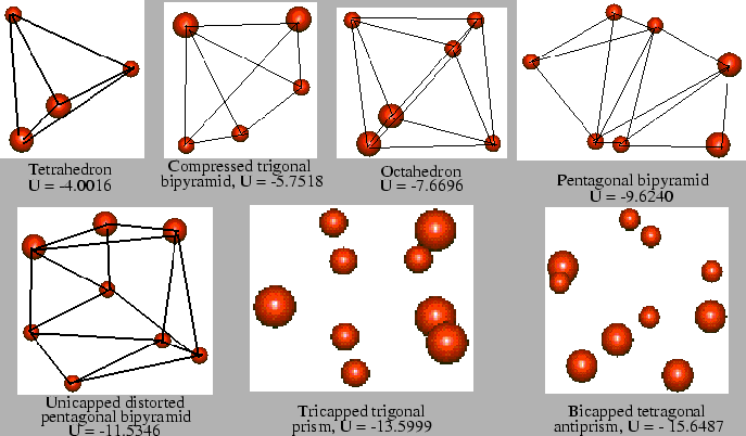Figure 5: Example of single GA run for 6 atom cluster.

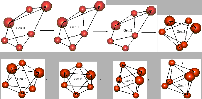Figure 6: Example of a single GA run for 7 atom cluster.

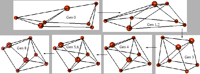Figure 7: Minimum population size required to reach the global optima for different cluster sizes.

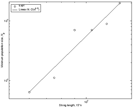Figure 8: Convergence time to reach the global optima for different cluster sizes.

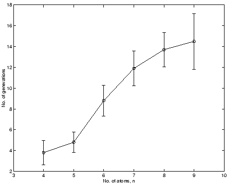Figure 9: Number of function evaluations required to reach the global optima for different cluster sizes.