ECE 486 Control Systems
Lecture 2
State-Space Representation of a System
State-Space Model – a Unified Framework
Recall from last time, we introduced the basic concept of control diagram, where the terminology we used include
- System input (\(R\))
- System output (\(Y\))
- Controller block (\(C\))
- Plant block (\(P\) or \(\tilde{P}\) for plant and actuator combined)
- Feedback loop (\(F\))
We also discussed the situation where the controller gain \(C\) (at the moment proprotional gain only) is large, we can achieve good reference tracking since \(C \to \infty\) implies \(Y \to R\). At the same time, the contribution of disturbance inputs \(D_1\) and \(D_2\) to the system output is minimal, we call it good disturbance rejection.
Now for a brief moment, we will look at another way of describing system dynamics – the state-space model. First off, a few quick examples.
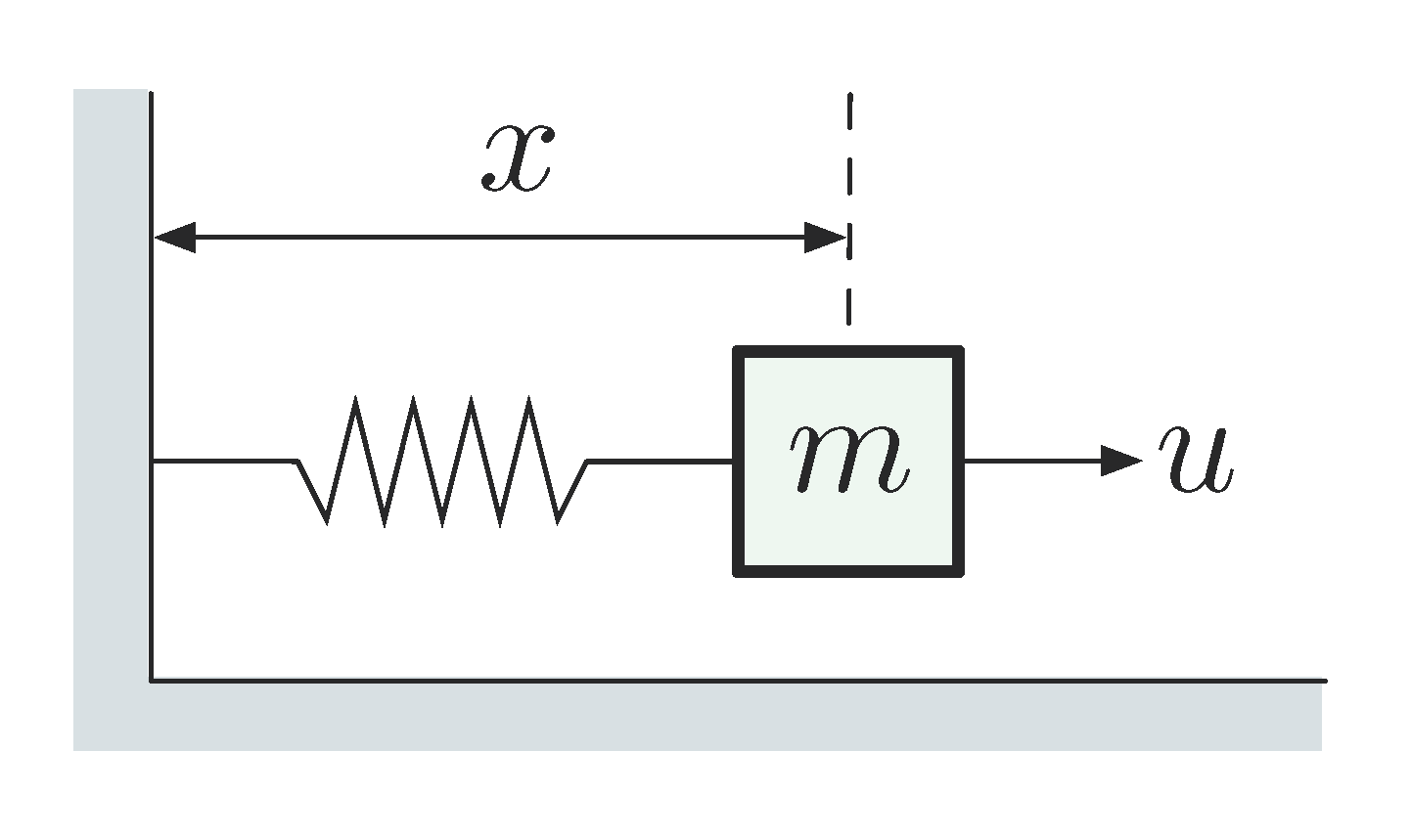
Example 1: Consider the Mass-Spring system as in Figure 1. Derive the governing differential equation and rewrite it in matrix form by reducing a higher order ODE to a set of first order ones.
Correction: The displacement \(x\) in the figure should be interpreted as measured against the resting position (\(x = 0\)) of the spring, not against the wall. Since a spring can be stretched also compressed.

Figure 1: Example 1 – Mass-Spring system
Solution: By Newton’s second law, total force equals mass times acceleration. Therefore in this case,
\begin{align*} \underbrace{F}_{\text{total force}} &= ma \\ &=\text{spring force} + \text{friction} + \text{external force}, \end{align*}where
\begin{align*} \mbox{spring force } &= -kx \quad \mbox{(by Hooke's law)} \\ \mbox{friction force } &= -\rho\dot{x} \quad \mbox{(by Stokes' law, linear drag pegged to velocity)}, \end{align*}i.e., we have the governing equation
\begin{align*} { -kx - \rho \dot{x} + u = m\ddot{x} }. \end{align*}We can move \(x\),\(\dot{x}\),\(\ddot{x}\) to one side, leaving \(u\) on the other, and normalize the leading coefficient,
\begin{align*} \ddot{x} + \frac{\rho}{m}\dot{x} + \frac{k}{m}x = \frac{u}{m}. \end{align*}This gives us a second order linear ODE.
To rewrite it in canonical form, we convert it to a system of first order ODEs by introducing veloctiy variable \(v = \dot{x}\),
\begin{align} \label{d2_eq1} \left\{ \begin{array}{ll} \dot{x} = v \hspace{5cm} \text{(by definition of velocity)} \\ \dot{v} = - \frac{\rho}{m}v - \frac{k}{m}x + \frac{1}{m}u \end{array} \right. . \end{align}Equation \eqref{d2_eq1} can also be written as (in order to see the matrix form more easily)
\begin{align*} \left\{ \begin{array}{lrrrrr} \dot{x} =& (0)x &+ &(1) v &+& (0) u \\ \dot{v} =& (- \frac{k}{m})x &+ &(- \frac{\rho}{m})v &+& (\frac{1}{m})u \end{array} \right. . \end{align*}Finally, we can express it in matrix form,
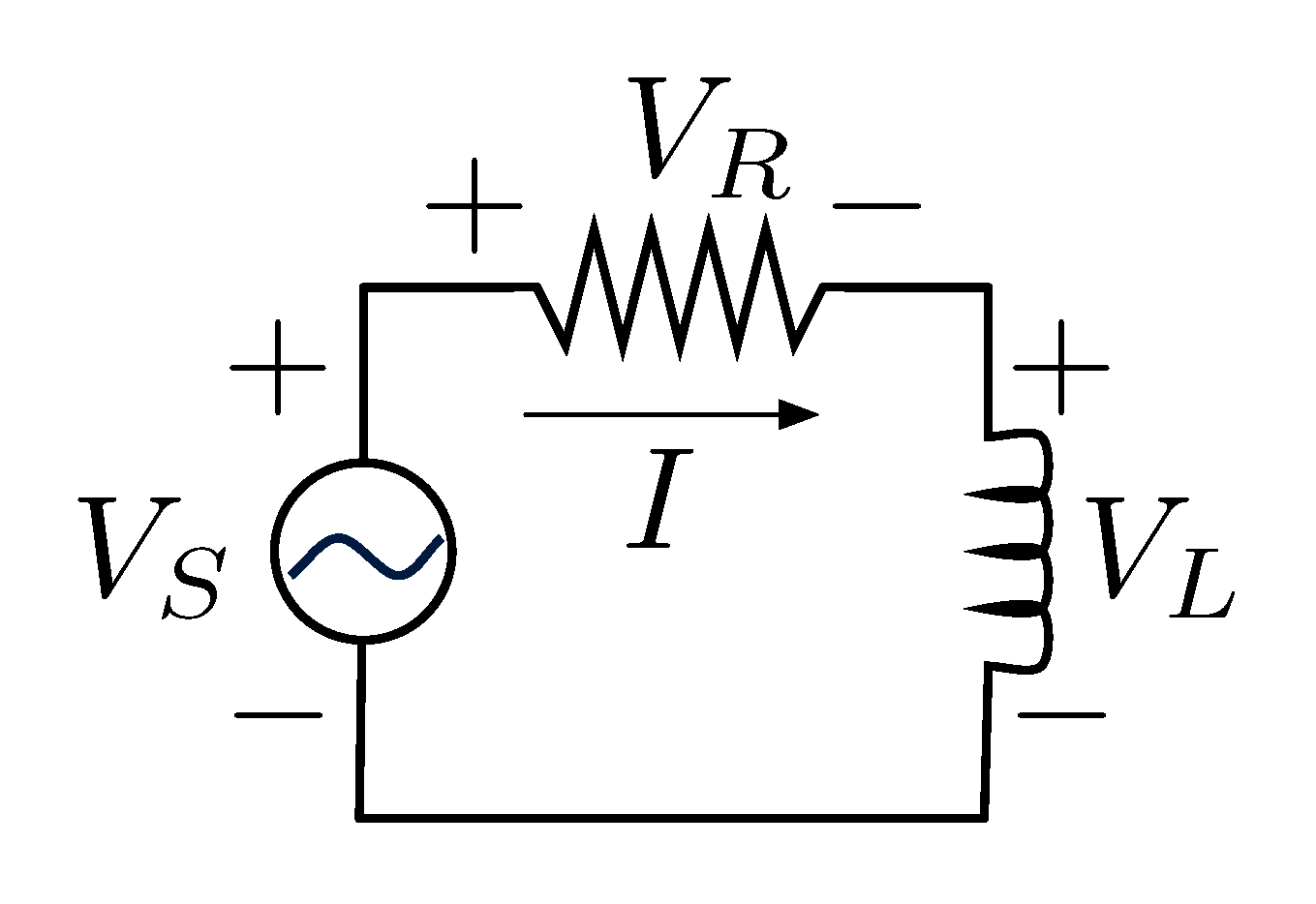
\begin{align*} \left(\begin{matrix} \dot{x} \\ \dot{v} \end{matrix}\right) &= \left( \begin{matrix} 0 & 1 \\ -\frac{k}{m} & -\frac{\rho}{m} \end{matrix}\right) \left(\begin{matrix} x \\ v\end{matrix}\right) + \left(\begin{matrix} 0 \\ \frac{1}{m} \end{matrix}\right)u. \end{align*}Example 2: Consider RL circuit as in Figure 2. Derive the governing differential equation and rewrite it in matrix form by reducing a higher order ODE to a set of first order ones.

Figure 2: Example 2 – RL circuit
Solution: We can largely repeat what we did in Example 1 but instead apply Kirchhoff’s voltage law, total voltage drop along the circuit loop is \(0\).
\begin{array}{rll} - V_S + V_R + V_L &=\, 0, & \text{(by Kirchhoff's voltage law)} \\ V_R &= \,RI, & \text{(by Ohm's law)} \\ V_L &= \,L\dot{I}. &\text{(by Faraday's law)} \end{array}Therefore, we have \({-V_S + RI + L\dot{I} = 0}\).
\begin{align*} \dot{I} = -\frac{R}{L}I + \frac{1}{L}V_S. \end{align*}Note this is a first order system.
General $n$-Dimensional State-Space Model
If we apply abstraction to both Example 1 and Example 2 above, for a system with \(n\) states and \(m\) inputs,
\begin{align*} \text{state } x = \left( \begin{matrix} x_1 \\ \vdots \\ x_n \end{matrix}\right) \in \RR^n, \qquad \text{input } u = \left( \begin{matrix} u_1 \\ \vdots \\ u_m \end{matrix}\right) \in \RR^m, \end{align*}a linear state space representation is a set of ODEs in matrix form
\begin{align*} \left( \begin{matrix} \dot{x}_1 \\ \vdots \\ \dot{x}_n \end{matrix}\right) = \left( \begin{matrix} {\Huge A} \\ \\ {\text{$n \times n$}\atop\text{matrix}}\end{matrix}\right) \left(\begin{matrix} x_1 \\ \vdots \\ x_n \end{matrix}\right) + \left( \begin{matrix} {\Huge B} \\ \\ {\text{$n \times m$}\atop\text{matrix}}\end{matrix}\right) \left(\begin{matrix} u_1 \\ \vdots \\ u_m \end{matrix}\right). \end{align*}Or for short,
\[\dot{x} = A_{n\times n}x + B_{n \times m}u.\]
This is called the dynamics equation of the state-space representation. Sometimes we can augment this dynamics equation with output equation. Denote the \(p\) outputs as a vector \(y\),
\begin{align*} \text{output } y &= \left( \begin{matrix} y_1 \\ \vdots \\ y_p \end{matrix}\right) \in \RR^p, \qquad y = Cx, \end{align*}where \(C\) is a \(p \times n\) matrix. For example, if we only care about (or can only measure) \(x_1\), then
\begin{align*} y = x_1 = \left( \begin{matrix} 1 & 0 & \ldots & 0 \end{matrix} \right)\left( \begin{matrix} x_1 \\ x_2 \\ \vdots \\ x_n \end{matrix}\right). \end{align*}The state-space representation of a system can be written as
\begin{align*}\dot{x} &= Ax + Bu,\\ y &= Cx. \end{align*}State-space models are useful and convenient for writing down system models for different types of systems, in a unified manner.
We will use the classic example of a simple pendulum to illustrate how to work with state-space models.
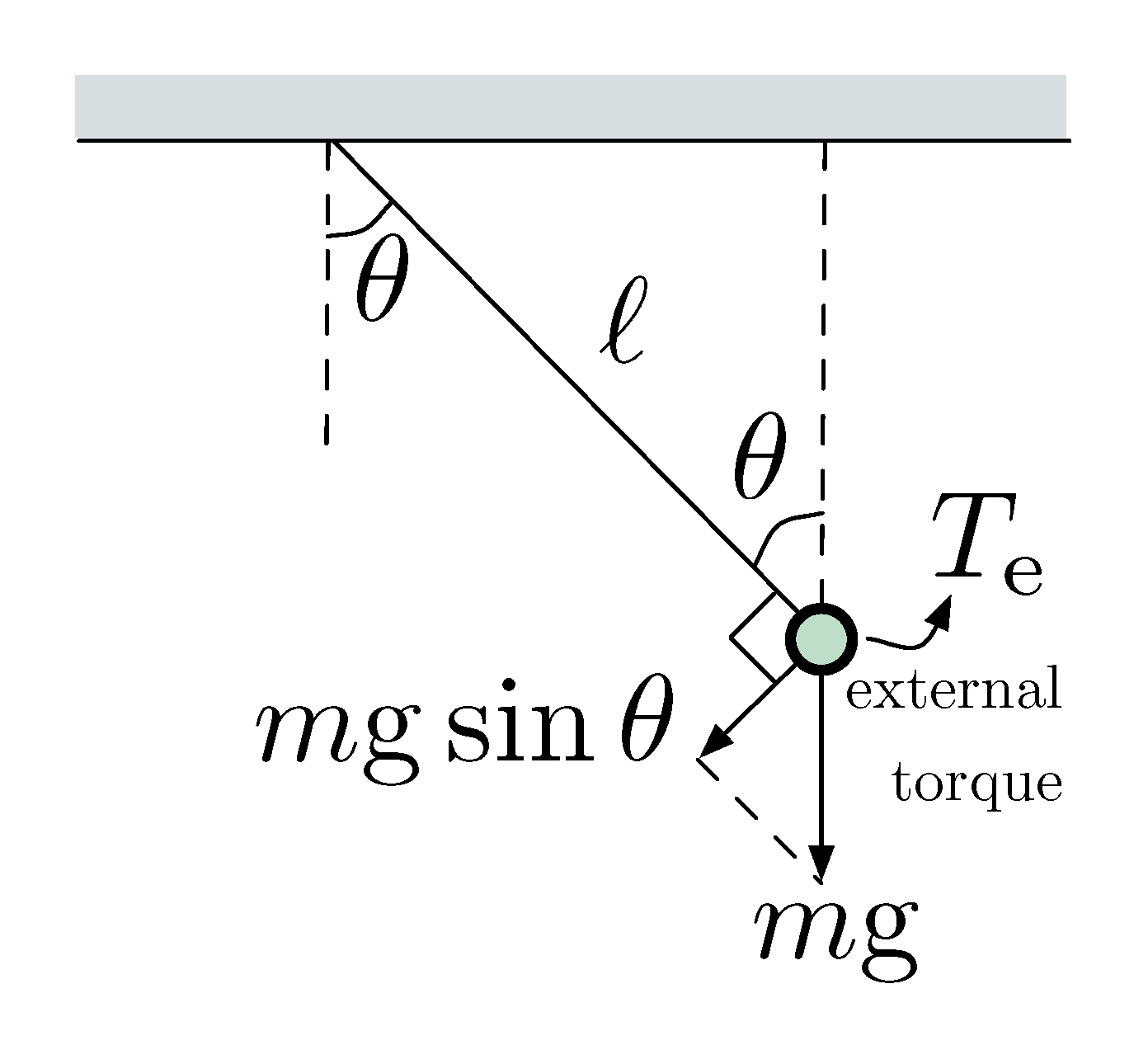
Example 3: Consider the simple pendulum as in Figure 3. Derive the governing differential equation and write it in the state-space representation.

Figure 3: Example 3 – Simple pendulum
Solution: Similar to Example 1, we apply here Newton’s second law but in its rotational version. It says total torque equals moment of inertia times angular acceleration.
\begin{align*} T &= J \alpha \\ \text{(pendulum torque } + \text{ external torque} &= \text{inertia} \times \text{angular acceleration),} \end{align*}where
\begin{align*} \text{pendulum torque} &= \underbrace{-m {\rm g} \sin \theta}_{\text{force}} \times \underbrace{\ell}_{\text{lever arm}},\\ \text{moment of inertia } J &= m\ell^2. \end{align*}By substitution,
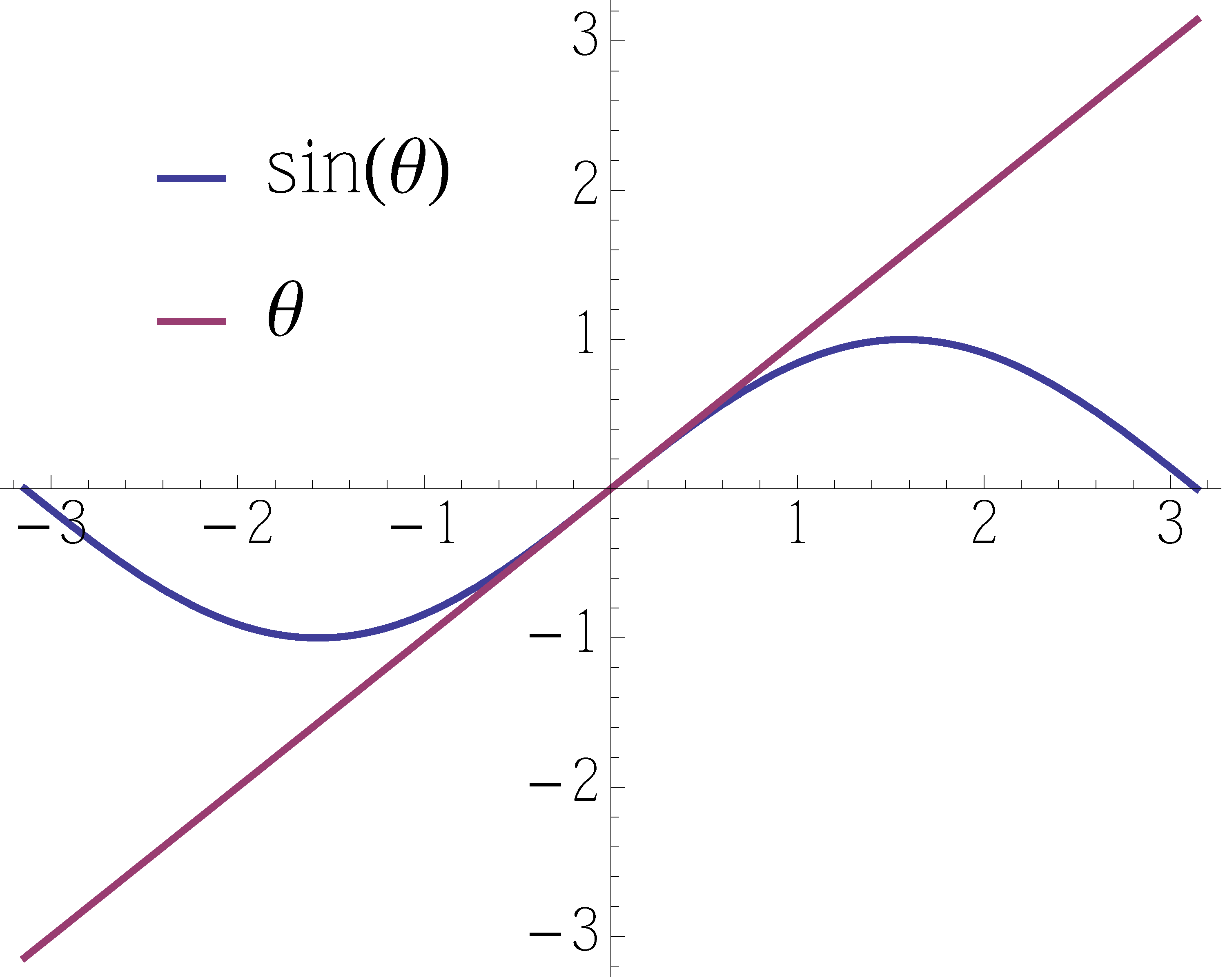
\begin{align} \label{d2_eq2} \ddot{\theta} &= - \frac{{\rm g}}{\ell}\sin \theta + \frac{1}{m\ell^2}T_{\rm e}. \end{align}It is a nonlinear equation though. Recall for small \(\theta\), use the approximation \(\sin \theta \approx \theta\) in Equation \eqref{d2_eq2},

Figure 4: Overlaid \(\sin x\) and \(x\)
We get
\begin{align} \label{d2_eq3} \ddot{\theta} &= - \frac{{\rm g}}{\ell} \theta + \frac{1}{m\ell^2}T_{\rm e}. \end{align}Repeat what we did at the end of Example 1 to rewrite Equation \eqref{d2_eq3} in state-space form: we introduce \(\theta_1 = \theta,\,\, \theta_2 = \dot{\theta}\), then
\begin{align*} \dot{\theta}_2 &= - \frac{{\rm g}}{\ell} \theta + \frac{1}{m\ell^2} T_{\rm e} \\ &= -\frac{{\rm g}}{\ell}\theta_1 + \frac{1}{m\ell^2}T_{\rm e}. \end{align*}So the state-space representation of a simple pendulum is
\begin{align*} \left( \begin{matrix} \dot{\theta}_1 \\ \dot{\theta}_2 \end{matrix} \right) = \left( \begin{matrix} 0 & 1 \\ -\frac{{\rm g}}{\ell} & 0 \end{matrix} \right) \left( \begin{matrix} {\theta}_1 \\ {\theta}_2 \end{matrix} \right) + \left( \begin{matrix} 0 \\ \frac{1}{m\ell^2} \end{matrix} \right)T_{\rm e}. \end{align*}Question: What if \(\theta\) is not small? say, \(\theta\) is around \(\pi\).
Answer: \(\sin \theta \approx \pi - \theta\) if \(\theta\) is around \(\pi\). (Why?)
Linearization of State-Space Models
Though in Example 3 we used the trick \(\sin x \approx x\) around \(x\) to obtain the linear state-space model, we are wondering if there is a general strategy to linearize state-space model. The answer is using Taylor series. Recall Taylor series expansion in one variable,
\begin{align*} f(x) &= f(x_0) + f'(x_0)(x-x_0) + \frac{1}{2}f''(x_0)(x-x_0)^2 + \ldots \\ &\approx f(x_0) + f'(x_0)(x-x_0). \hspace{2cm} \text{(linear approximation around $x=x_0$)} \end{align*}For a general nonlinear control system
\begin{align*} & \dot{x} = f(x,u) &\text{(nonlinear state-space model)} \\ & x = \left( \begin{matrix} x_1 \\ \vdots \\ x_n\end{matrix}\right), \quad u = \left( \begin{matrix} u_1 \\ \vdots \\ u_m \end{matrix}\right), \quad f = \left( \begin{matrix} f_1 \\ \vdots \\ f_n \end{matrix}\right), \end{align*}we can apply Taylor expansion in multivariables. Assume \(x=0\),\(u=0\) is an equilibrium point: \(f(0,0) = 0\), i.e., when the system is at rest and no control is applied, the system does not move. Around \((x,u)=(0,0)\), for each \(f_i(x, u)\) of \(f(x,u)\), \(i=1,\ldots,n\),
\begin{align*} f_i(x,u) = \underbrace{f_i(0,0)}_{=0} &+ \frac{\partial f_i}{\partial x_1}(0,0)x_1 + \ldots + \frac{\partial f_i}{\partial x_n}(0,0) x_n \\ &+ \frac{\partial f_i}{\partial u_1}(0,0)u_1 + \ldots + \frac{\partial f_i}{\partial u_m}(0,0) u_m. \end{align*}After we assemble those \(n\) equations, we get the linearized state-space model
\[ \dot{x} = Ax + Bu, \text{ where $A_{ij} = \frac{\partial f_i}{\partial x_j} \Bigg|_{x=0 \atop u=0},\,\, B_{ik} = \frac{\partial f_i}{\partial u_k} \Bigg|_{x=0 \atop u=0}$}. \] \(A\) is nothing but the Jacobian of \(f(x,u)\) w.r.t. \(x\) at equilibrium and similarly \(B\) is the Jacobian of \(f(x,u)\) w.r.t. \(u\) at equilibrium.
Important: Since we have ignored the higher-order terms, this linear system is only an approximation that holds only for small deviations from equilibrium.
Let’s use the general strategy instead of a trick to relinearize the nonlinear dynamics of a simple pendulum in Example 3.
Example 3 (revisted): Relinearize the state-space model of a simple pendulum in Example 3 above.
Solution: The original nonlinear state-space model:
\begin{align*} \dot{\theta}_1 &= f_1(\theta_1,\theta_2,T_{\rm e}) = \theta_2, \hspace{5cm} \text{(already linear)}\\ \dot{\theta}_2 &= f_2(\theta_1,\theta_2,T_{\rm e}) = -\frac{{\rm g}}{\ell} \sin \theta_1 + \frac{1}{m\ell^2} T_{\rm e}. \end{align*}Linearize \(f_2\) around equilibrium \((\theta_1,\theta_2,T_{\rm e}) = (0,0,0)\):
\begin{array}{rlrlrl} \frac{\partial f_2}{\partial \theta_1} &=\, - \frac{{\rm g}}{\ell} \cos \theta_1, & \frac{\partial f_2}{\partial \theta_2} &=\, 0, \qquad \frac{\partial f_2}{\partial T_{\rm e}} &\,= \frac{1}{m\ell^2}, \\ \frac{\partial f_2}{\partial \theta_1}\Bigg|_0 &=\, - \frac{{\rm g}}{\ell}, & \frac{\partial f_2}{\partial \theta_2}\Bigg|_0 &\,= 0, \qquad \frac{\partial f_2}{\partial T_{\rm e}}\Bigg|_0 &=\, \frac{1}{m\ell^2}. \end{array}Therefore the linearized state-space model of the pendulum is
\begin{align*} \dot{\theta}_1 &= \theta_2,\\ \dot{\theta}_2 &= - \frac{{\rm g}}{\ell} \theta_1 + \frac{1}{m\ell^2}T_{\rm e}, \end{align*}which is the same as Example 3.
General Linearization Procedure
Note that if systems have different equilibria other than \((x, u) = (0,0)\), we may apply translation to shift nonzero equilibrium to the origin:
\begin{align*} &\underline{x} = x-x_0, \qquad \underline{u} = u - u_0, \\ &\underline{f}(\underline{x},\underline{u}) = f(\underline{x} + x_0, \underline{u} + u_0) = f(x,u). \end{align*}Since \(\dot{\underline{x}} = \underline{f}(\underline{x},\underline{u})\) is a system with origin as its equilibrium, we can apply the aforementioned linearization method we discussed for such systems. After we compute Jacobians and formulate the linearization in terms of \(\underline{x}\) and \(\underline{u}\), we substitute \(\underline{x} = x-x_0\), \(\underline{u} = u - u_0\) to get a linearized model in terms of \(x\) and \(u\).
Observation: For any linear system, it must have an equilibrium point at \((x,u) = (0,0)\) since if \(f\) is already linear
\begin{align*} f(x,u) = Ax + Bu \xrightarrow{x = 0,~u = 0} f(0,0) = A0 + B0 = 0. \end{align*}