ECE 486 Control Systems
Lecture 12
Lead and Lag Compensators
Last time we finished the discussion of rules for sketching root loci. (Rules E — F in Lecture 11; Rules A — D in Lecture 10.) We also introduced dynamic compensation to approximate PD control.
Important: Rules A — F as discussed in class is a highlighted subset of a larger set of rules for sketching root locus. See FPE or Wikibooks 11 Root Locus Rules for details.
The most frequently inquired ones during office hours are breakaway points on real axis, origin of asymptotes and departure angles at open loop poles and arriving angles at open loop zeros, proof (outline) of which shall be given below.
Show breakaway (or reentry) points are given by \(\frac{\d L(s)}{\d s} = 0\).
Sketch of Proof: We need to exploit the fact when different branches meet at some breakaway (or reentry) point \(s_0\), that point is a repeated root of characteristic equation.
\[ 1 + K_0 L(s_0) = 0 \tag{*.1} \label{d12_*eq1}\]
for some \(K_0 > 0\) and \(s_0 \in \RR\). Equation \eqref{d12_*eq1} can be rewritten as \(L(s_0) = -\frac{1}{K_0}\). Since \(s_0\) is a repeated root, \(\frac{\d L(s)}{\d s} = 0\) at \(s = s_0\), i.e., \(s_0\) solves the equation
\[\frac{\d L(s)}{\d s} = 0.\]
Show the origin of asymptotes is given by \(\alpha = \frac{\sum_{i=1}^n p_i - \sum_{j=1}^m z_j}{n - m}\) when the degrees of \(a(s)\) and \(b(s)\) differ by \(2\) or more.
Sketch of Proof: Let \(a(s)\), \(b(s)\) be as usual,
\begin{align*} a(s) &= a^n + a_1 s^{n-1} + \cdots,\\ b(s) &= b^m + b_1 s^{m-1} + \cdots. \end{align*}By Vieta’s formula, \(\sum_i p_i = -a_1\) and \(\sum_j z_j = -b_1\). Let \(r_1, r_2, \ldots, r_n\) be the closed loop poles, i.e., they solve the characteristic equation
\[ a(s) + K b(s) = 0.\]
Since the \(\deg (a(s)) - \deg (b(s)) = n - m \geq 2\),
\[ -a_1 = \sum_i r_i = \sum_i p_i. \tag{*.2}\label{d12_*eq2}\]
But when \(K \to \infty\), root locus at infinity means \(m\) of \(r_i\)’s approach corresponding \(m\) open loop zeros; the remaining \(n - m\) closed loop poles \(r_i\)’s approach \(\alpha\), making \(\alpha\) a closed loop pole of order \(n - m\). Then Equation \eqref{d12_*eq2} becomes,
\[ (n-m)\alpha + \sum_j z_j = \sum_i p_i.\]
Divide out \((n-m)\) on both sides, we prove the claim.
Show angle of departure at an open loop pole \(p_0\) is given by
\[\varphi_{p_0} = 180^\circ - \sum_{p_i \neq p_0} \angle{(p_0 - p_i)} + \sum_j \angle{(p_0 - z_j)}. \]
Similarly, angle of arrival at an open loop zero \(z_0\) is given by
\[\varphi_{z_0} = 180^\circ + \sum_i \angle{(z_0 - p_i)} - \sum_{z_j \neq z_0} \angle{(z_0 - z_j)}. \]
Sketch of Proof: This is simply the application of phase condition around the pole or zero of interest. The trick used here is to draw a tiny circle around the pole or zero, then apply the phase condition.
In this lecture, we will give more details about the use of lead and lag dynamic compensators for approximate implementation of PD and PI control.
Recall the diagram of dynamic compensation,

Figure 1: Dynamic compensation for double integrator
The corresponding characteristic equation is
\[ \tag{1} \label{d12_eq1} 1 + K \cdot \underbrace{\dfrac{s+z}{s+p} \cdot \dfrac{1}{s^2}}_{:=L(s)} = 1 + KL(s) = 0. \]
In Figure 1, the controller of the form
\[ K \frac{s+z}{s+p} \text{, where $K,z,p > 0$ are design parameters,} \]
is a lead or lag compensator.
Whether it is lead or lag depends on the relative values of \(z\) and \(p\),
- it is a lead compensator if \(z < p\);
- it is a lag compensator if \(z > p\).
Why the name “lead/lag”? Indeed, think of \(s = j\omega\) in frequency response
\begin{align*} \angle \frac{j\omega + z}{j\omega + p} &= \angle (z + j\omega) - \angle (p + j\omega)\\ &= \psi - \phi. \tag{2} \label{d12_eq2} \end{align*}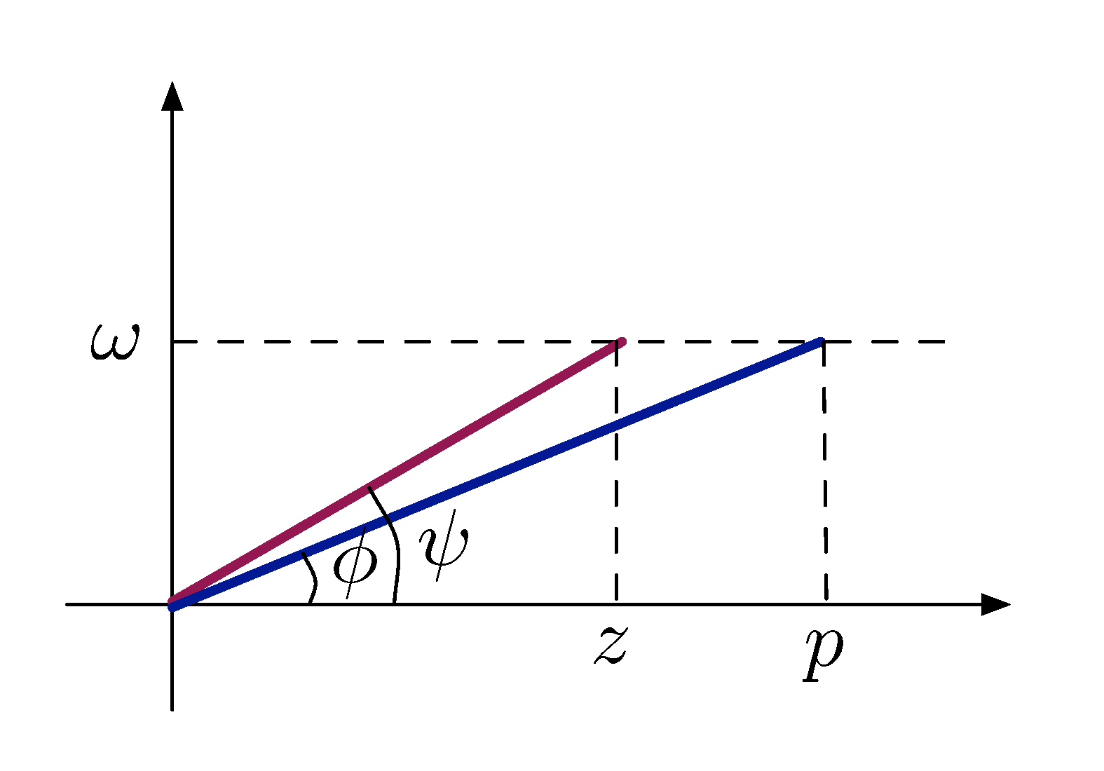
Figure 2: Naming of Lead/Lag compensator
From Figure 2 and Equation \eqref{d12_eq2}, it is natural to note
- if \(z < p\), then \(\psi - \phi > 0\), hence a phase lead;
- if \(z > p\), then \(\psi - \phi < 0\), hence a phase lag.
Lead Compensator Applied to Double Integrator
Recall from last time as shown in Figure 1, a dynamic compensator approximating PD control
\[K \dfrac{s+z}{s+p} \tag{3} \label{d12_eq3} \]
was applied to a double integrator, where \(K = K_{\rm P} + pK_{\rm D}\) and \(z = \frac{pK_{\rm P}}{K_{\rm P} + pK_{\rm D}}\). Note as \(p \to \infty\), \(z \to \frac{K_{\rm P}}{K_{\rm D}}\) which is a constant. Therefore the dynamic compensator approximating PD control in Equation \eqref{d12_eq3} is a lead controller.
To keep things simple, let’s set \(K_{\rm P} = K_{\rm D}\). Then
\begin{align*} K &= K_{\rm P} + pK_{\rm D} = (1+p)K_{\rm D}, \\ z &= \frac{pK_{\rm P}}{K_{\rm P} + pK_{\rm D}} \\ &= \frac{pK_{\rm D}}{(1+p)K_{\rm D}} \\ &= \frac{p}{1+p} \\ &\to 1, \text{ as } p \to \infty. \end{align*}Since we can choose \(p\) and \(z\) directly, let’s take \[ z=1 \text{ and large } p. \]
We expect controller in Equation \eqref{d12_eq3} to be similar to PD control.
Now we want to try a few numerical values of \(p\) with \(z\) fixed as \(1\). The equivalent open loop transfer function \(L(s)\) in Equation \eqref{d12_eq1} then becomes
\begin{align*} L(s) &= \frac{s+z}{s+p} \cdot \frac{1}{s^2} \\ &= \frac{s+1}{s^2 (s+p)}. \end{align*}Setting \(p = 10\), we obtain the root locus plot with \(L(s)\) as shown in Figure 3.
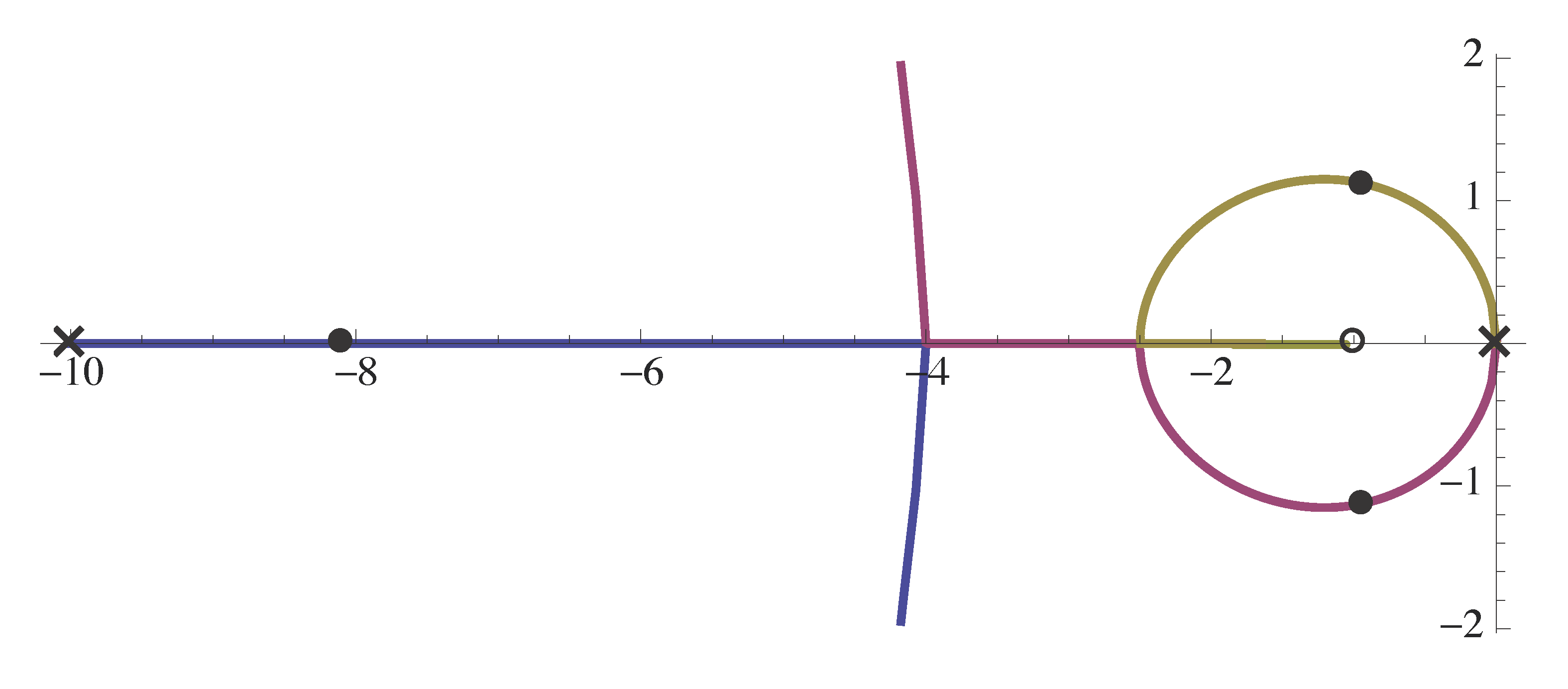
Figure 3: Root locus plot with \(L(s) = \frac{s+1}{s^2 (s+p)}\) and \(p = 10\)
Based on Figure 3, we see that close to $jω$-axis, root locus looks similar to the root locus of PD control (Fig. 8, Lecture 11). However, the pole at \(s=-10\) makes the locus look different when root locus is far into Left Half Plane.
However Figure 3 seems to show the design looks good — it may have nice damping; it can meet reasonable specifications.
Is there any concerns with large values of \(p\)? We used large \(p\) to approximate PD control so that we addressed the lack of causality. But it is still subject to noise amplification since we are very close to PD control when \(p\) is large.
Let’s continue our numerical experiments. Try \(p = 5\).
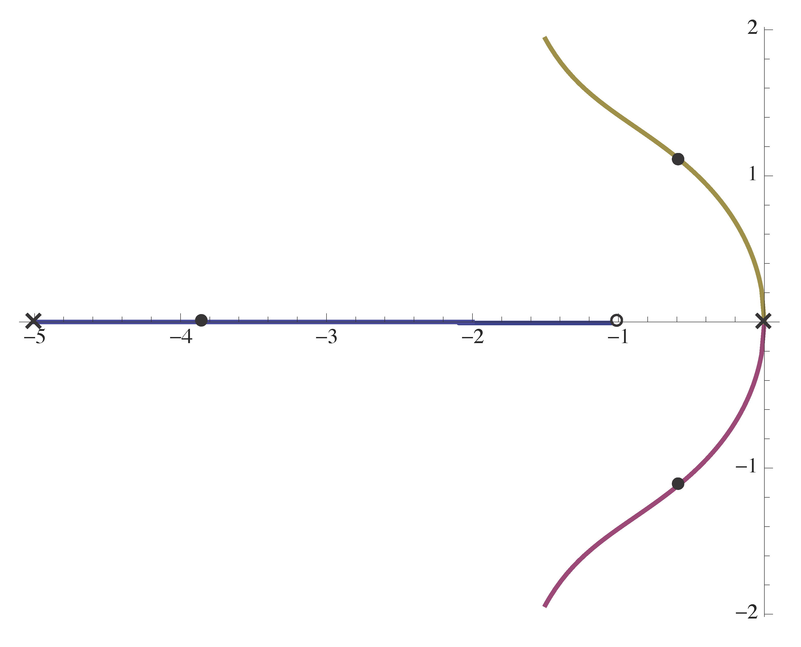
Figure 4: Root locus plot with \(L(s) = \frac{s+1}{s^2 (s+p)}\) and \(p = 5\)
For this value of \(p = 5\), the root locus in Figure 4 is very different from the previous case \(p = 10\); it is not nearly as nicely damped as for \(p=10\).
This prompt us into trying some \(p\) in between \(p=5\) and \(p=10\), say \(p = 9\).
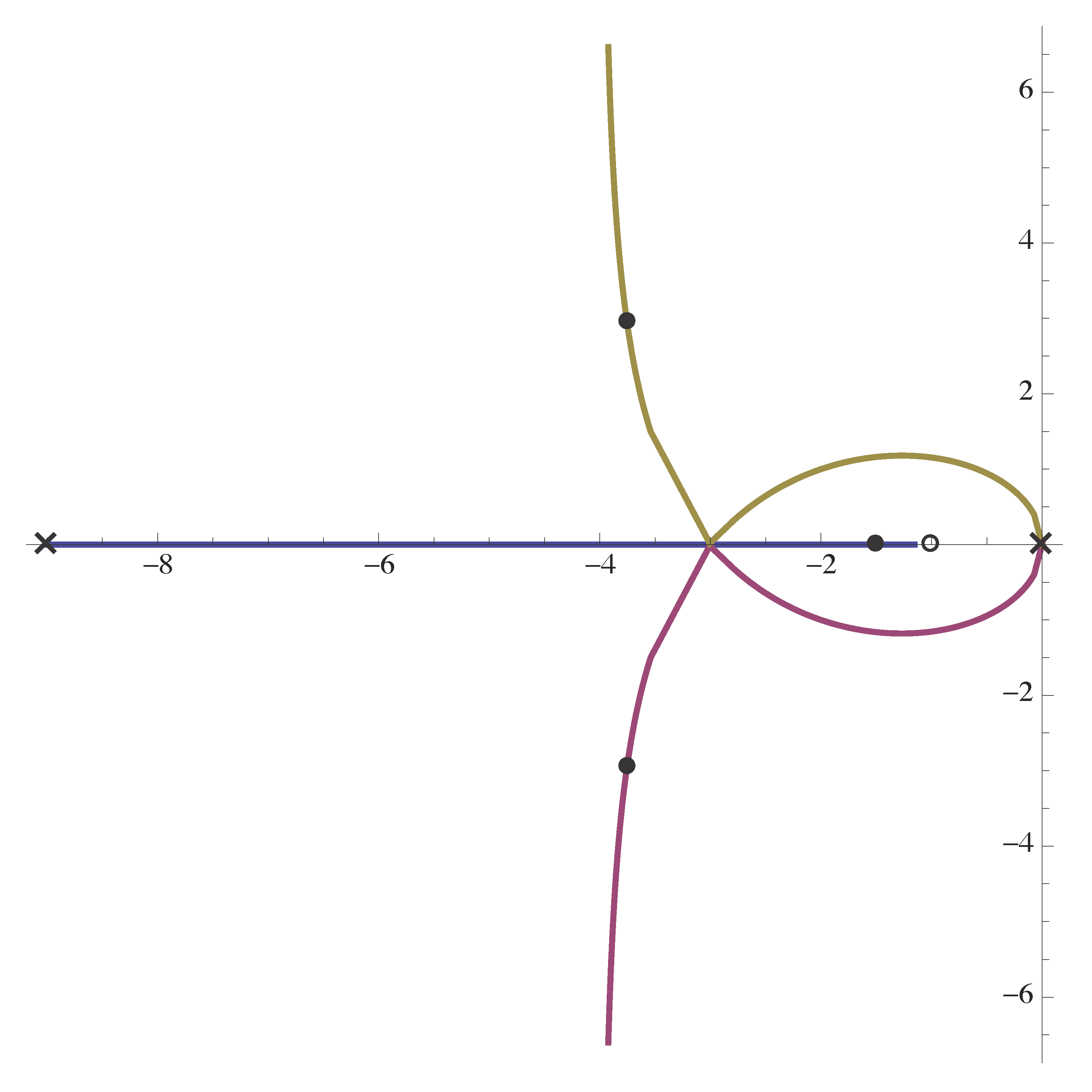
Figure 5: Root locus plot with \(L(s) = \frac{s+1}{s^2 (s+p)}\) and \(p = 9\)
When \(p = 9\), the branches in Figure 5 meet or break in and separate or break away at the same point on the real axis.
Summary on Design Trade-offs: From what we have seen so far,
- for large \(p\), Figure 3 shows that the root locus can have good damping, but bad noise suppression (too close to PD control); the branches first break in (meet at the real axis), then break away;
- for small \(p\), Figure 4 shows that noise suppression is better (since \(p\) is small, hence not large, not close to PD control), but the root locus could be overall close to $jω$-axis, which does not give good damping; there is no break-in for small values of \(p\);
- for \(p\) somewhere between, Figure 5 shows in this case the root locus is some transition between the two aforementioned types; the break-in and break-away points are the same.
Lead Controller Design
In the previous discussion, with a lead controller in place, we had
\[ KL(s) = K \frac{s+z}{s+p} \cdot G_p(s), \]
where the lead zero parameter \(z\) and lead pole parameter \(p\) were constrained to satisfy \(z < p\).
In our example of controlling double integrator with \(G_p(s) = \frac{1}{s^2}\), we set \(z=1\) to approximate PD control. Then \(p > 1\) was our design parameter. \(K\) was the varying gain parameter in the root locus.
Conversely, we can assume that \(p\) is given (say, from some noise suppression considerations), and we look for \(z\) such that this combination of \(p, z\) will give us a desired pole on the root locus.
Now we ask the question, is there a systematic procedure for doing this?
Pole Placement Using Root Locus
Recall our example of double integrator with lead compensation, \[ \tag{4} \label{d12_eq4} KL(s) = K \frac{s+z}{s+p} \cdot \frac{1}{s^2}. \]
Consider the following problem.
Problem: Given \(p\) and a desired closed-loop pole \(s\), find the value of \(z\) that will guarantee this (if possible).
Solution: Apply the phase condition \(\angle L(s) = 180^{\circ}\) to \(L(s)\) in Equation \eqref{d12_eq4}.
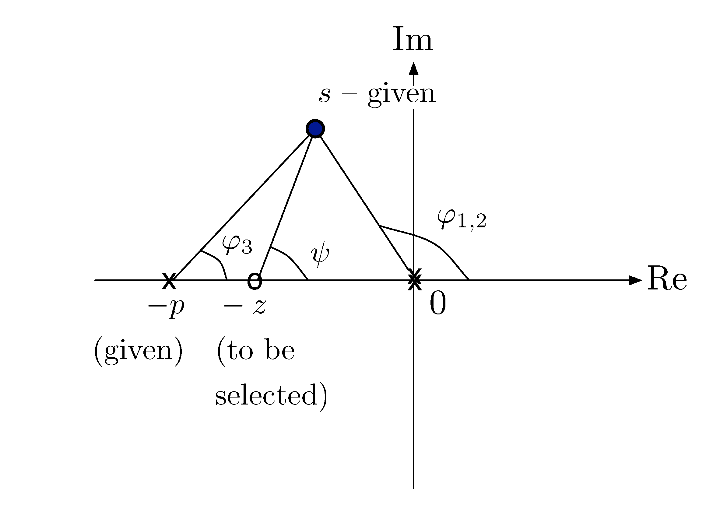
Figure 6: Find \(z\) with given \(p\) and a desired closed-loop pole \(s\)
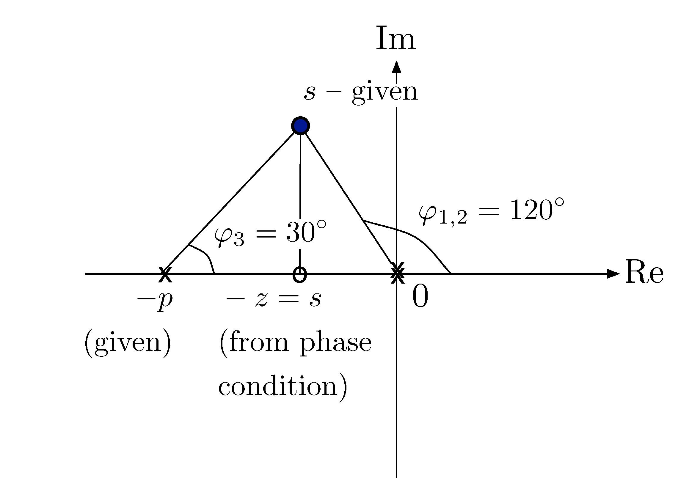
Figure 7: Find \(z\) with given \(\varphi_1 = \varphi_2 = 120^\circ\) and \(\varphi_3 = 30^\circ\)
Correction: In Figure 7, \(-z = {\rm Re}(s)\), not \(s\) itself.
For example, suppose \(\varphi_1 = \varphi_2 = 120^\circ\), \(\varphi_3 = 30^\circ\).
\begin{align*} \psi &= 180^\circ + \sum_i \varphi_i \\ &= 180^\circ + 120^\circ + 120^\circ + 30^\circ \\ &= 450^\circ \\ &= 90^\circ \bmod 360^\circ \end{align*}Thus, we should have \(z = -{\rm Re}(s)\).
Control Design Using Root Locus (Continued)
Consider an unstable plant transfer function \(G_p(s) = \dfrac{1}{s-1}\), we want to stabilize it with constant reference tracking.
In Lecture 9, we saw that for perfect steady-state tracking we may use PI control.

Figure 8: PI control for unstable plant \(G_p(s) = \dfrac{1}{s-1}\)
The closed-loop poles are determined by characteristic equation
\[ 1 + \underbrace{\left(K_{\rm P} + \frac{K_{\rm I}}{s}\right)}_{G_c(s)} \underbrace{\left(\frac{1}{s-1}\right)}_{G_p(s)} = 0. \]
To use the Root Locus Method, we convert it into the Evans form \(1 + KL(s) = 0\), where
\[ L(s) = \dfrac{b(s)}{a(s)} = \dfrac{s^m + b_1 s^{m-1} + \cdots}{s^n + a_1 s^{n-1} + \cdots} \]
is proper and rational.
Choose \(K = K_{\rm P}\) as the varying parameter. Further assuming \(K_{\rm I}/K_{\rm P}\) is fixed, say \(1\), rewrite the characteristic equation to obtain open loop \(L(s)\),
\begin{align*} 1 + \left(K_{\rm P} + \frac{K_{\rm I}}{s}\right)\frac{1}{s-1} &= 1 + \frac{K_{\rm P}s + K_{\rm I}}{s} \frac{1}{s-1} \\ & = 1 + K_{\rm P} \frac{s + K_{\rm I}/K_{\rm P}}{s(s-1)}\\ & = 1 + K \underbrace{\frac{s + 1}{s(s-1)}}_{:=L(s)}. \end{align*}With this \(L(s) = \frac{s + 1}{s(s-1)}\), let’s sketch the root locus of \(1 + KL(s)\).
- Rule A says there are \(2\) branches.
- Rule B says branches of root locus start at \(p_1 = 0\) and \(p_2 = 1\). Note \(p_2 = 1\) is on the Right Half Plane.
- Rule C says branches of root locus end at \(z_1 = -1\) and \(\pm \infty\).
- Rule D says the real locus is the union of intervals \([0,1]\) and \((-\infty,-1]\) on the real axis.
- Rule E says the only asymptote is with an angle at \(180^\circ\).
- Rule F is used to compute $jω$-crossings as follows.
The root locus is shown in Figure 9.
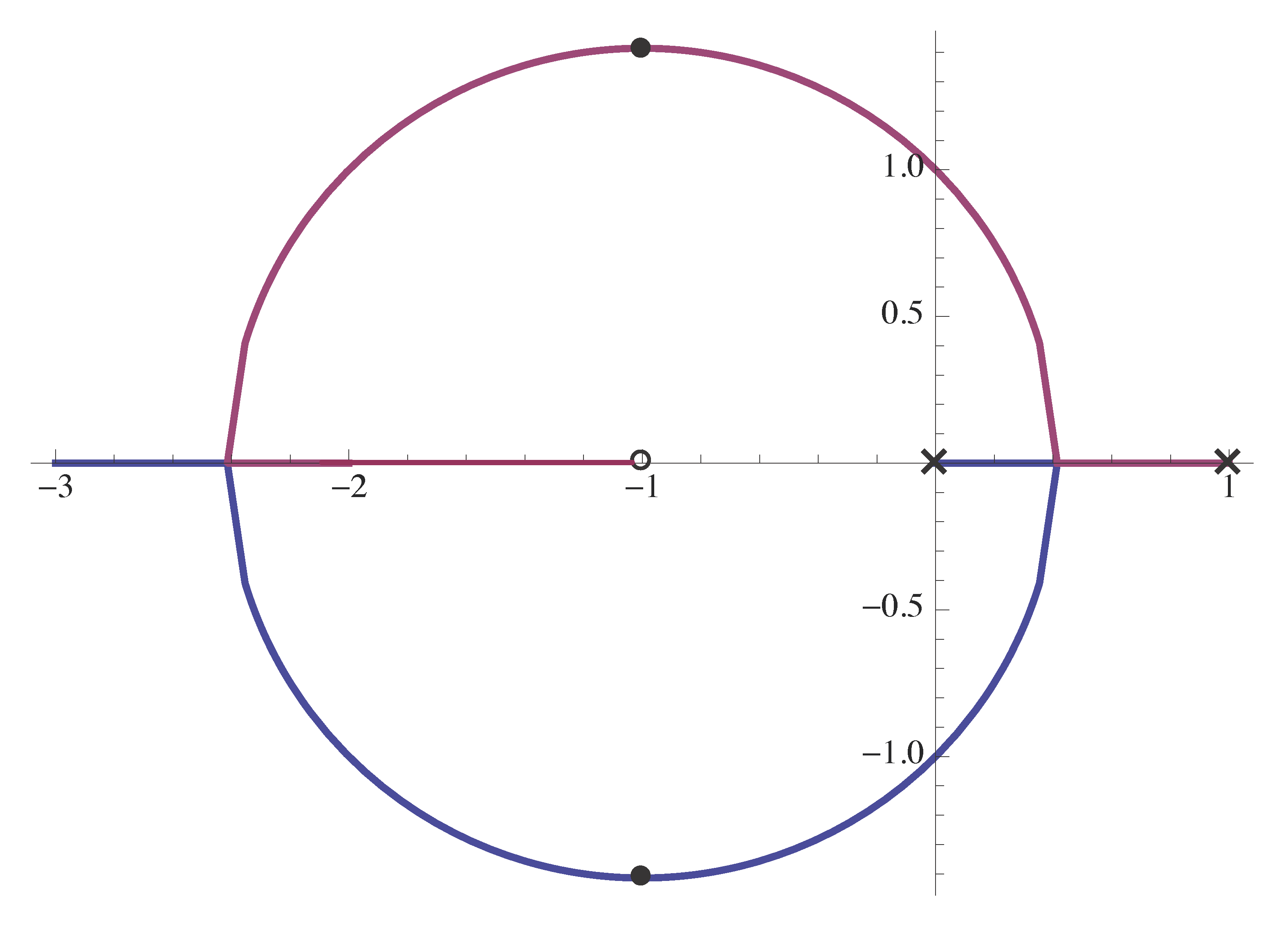
Figure 9: Root locus plot with \(L(s) = \frac{s + 1}{s(s-1)}\)
From the root locus plot, we conclude
- in order to obtain closed loop poles in the Open Left Half Plane, the system must be strictly stable; so \(K > 1\) by Routh-Hurwitz criterion applied to left hand side of Equation \eqref{d12_eq5};
- for very large \(K\), we get a completely damped system, i.e., \(\zeta > 1\) with negative real poles;
steady-state tracking of constant reference is perfect. Indeed
\begin{align*} \frac{E}{R}(s) &= \frac{1}{1+G_cG_p} \\ &= \frac{s(s-1)}{s(s-1) + K(s+1)}. \\ \end{align*}As long as \(K > 1\), stability is guaranteed. Then by Final Value Theorem, the DC gain of \(\frac{E}{R}(s) = 0\).
However, \(\frac{1}s\) itself is not a strictly stable element. So we want to approximate a PI controller with dynamic compensation like what we did as to PD control because of PD control not being causal.
Approximate PI via Dynamic Compensation
Here’s one idea,
\begin{align*} \text{replace } K \frac{s+1}{s} \quad \text{by} \quad K\frac{s+1}{s+p}, \text{ where $p$ is small}. \end{align*}More generally, if \(z = \frac{K_{\rm I}}{K_{\rm P}}\), then
\begin{align*} \text{replace } K \frac{s+z}{s} \quad \text{by} \quad K\frac{s+z}{s+p}, \text{ where $p < z$}. \end{align*}This is a lag compensation or lag control. We use lag controllers as dynamic compensators for approximating PI control. (cf. lead compensators for approximating PD control.)