Molecular Dynamics

The primary goal of this work is to develop a generalized KMC code, however it is also important to verify and demonstrate the functionality of the code after it is completed. In this study, the code is demonstrated by comparing using diffusivity results generated from KMC simulations of three different interatomic potentials. This requires not only an explanation of the KMC code developed, but also an explanation of the Molecular Dynamics simulations carried out to produce migration energies from the selected potentials.

For this study, molecular dynamics simulations were performed to determine local configuration dependent migration energies using the selected interatomic potentials.

Background

At the most basic level, Molecular Dynamics (MD) evolves an atomic system using Newton's classical equation of motion:

$$\vec{F} = m\vec{a}$$ (3.1)

The system is initialized to some initial state, where each particle in the system has an initial position and an initial velocity. Even without the presence of an external force field (e.x. gravity), each particle experiences some force due to its configurational potential energy:

$$\vec{F}\left(\vec{r}\right) = - \nabla V\left(\vec{r}\right)$$ (3.2)

In general, the form of this potential energy function could be arbitrarily complex, but in most cases the potential is simplified down to a two or three particle interaction. This is done primarily because of the computational expense of evaluating the potential energy function. In this study, the selected interatomic potentials are all pairwise interactions. The form of these potentials is given in Equation 2.5, with the corresponding fitted parameters given in Table 2.1. Once the form of the potential energy function is known, the corresponding force can be derived from Equation 3.2. The acceleration of each particle at a given time step can then be calculated by rearranging Equation 3.1:

$$\vec{a} = \frac{\vec{F}}{m}$$ (3.3)

Once the acceleration of each particle is known, an integrator is used to evolve the position and velocity of each of the particles in the system by one time step. One of the most popular integrators, which is also the integrator used by the code in this study, is the Verlet leapfrog algorithm given by:

$$\vec{r}(t+h) = \vec{r}(t)+ h\vec{v}\left(t+\frac{1}{2}h\right)$$ (3.4)

$$\vec{v}\left(t+\frac{1}{2}h\right) = \vec{v}\left(t-\frac{1}{2}h\right) + h \vec{a}(t)$$ (3.5)

where $t$ is the current time and $h$ is the time step used. The name ``leapfrog'' comes from the fact that the positions and velocities are calculated at staggered time steps, so the positions and velocities appear to ``leapfrog'' over each other. These calculates are fairly easy to evaluate, so most of the computational time from an MD simulation is spent in the evaluation of forces. Since the configurational force on a single particle depends on the position of every other particle in the system, evaluating this force is very computationally expensive especially as the complexity of the potential is increased.

Migration Energy Calculations

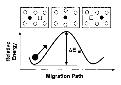
In order to calculate the oxygen vacancy migration energies from MD, a simulation volume consisting of $4 \times 4 \times 4$ conventional unit cells of CeO$_2$ (768 atoms) is used. Periodic boundary conditions are applied to this volume to extend the system infinitely in each direction, allowing for the calculation of bulk material properties by eliminating boundary surface effects. A vacancy defect is generated and a local dopant environment is created by substituting La dopant atoms as necessary at the appropriate neighboring cation sites (shown schematically in Figure 3.1). The defect energy is calculated for the system at varying points along the migration pathway ( so that the minimum (stable) energy and maximum (saddle-point) energy for the migration can be found. The migration energy for the configuration is then calculated as the difference between the saddle point energy and stable configuration energy.

Figure 3.1: Schematic representation of the migrating vacancy and local dopant environment used to model vacancy migration in La-doped CeO$_2$ [31]. The arrow shows the migration pathway of the oxygen atom (opposite pathway of the oxygen vacancy), the square shows the initial position of the vacancy after migration, and the 6 numbered cation sites show the local configuration sites that are considered.

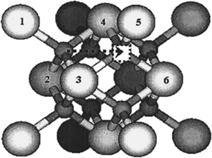Figure 3.2: Defect energy along the oxygen vacancy migration pathway [31]. Migration energy is calculated as the difference between the saddle point and minimum energies.

GULP Defect Energy Calculations

The MD simulations in this study are performed using the GULP (General Utility Lattice Program) code [32], which uses the Mott-Littleton approach [33] to estimate defect energies. In this approach, the environment around the defects is broken up into three regions by two concentric spheres. In the smallest concentric sphere (Region I), the ions are assumed to be strongly perturbed by the presence of defect and are explicitly relaxed with respect to their Cartesian coordinates. In the second concentric sphere (Region Ia), the ions are assumed to be weakly perturbed by the presence of the defect, so their displacements can be approximated. The area outside the second concentric sphere (Region IIb) is treated as a dielectric medium. Using this approach, both the energy minima (corresponding to stable defect configurations) and energy maximum (corresponding to the migration saddle point plane) can be considered. Since the migration energy is the difference between the saddle point energy and the stable configuration energy, the Mott-Littleton approach is very convenient for this work.

Since varying the Region I and Region II sizes strongly affects the defect energy calculation, it is important to be sure that the these sizes are chosen correctly. As the region sizes increase, the approximates made will become increasingly valid, but at the same time the computational cost will increase substantially. It is important to find a compromise between these two, as region sizes much be large enough that the defect energies are converged, but small enough to be computed in a reasonable amount of time. To find the best region sizes, the defect minimum and saddle point energies were calculated with varying region sizes in the two extreme dopant cases: will no nearest neighbor lanthanum dopant ions and with all six nearest neighbor dopant ions. These simulations were performed by Dr. Di Yun, using yttrium as the dopant, but the results are transferable to other dopant cases. The results of these simulations are given in Table 3.1. These results show that defect energy drops with increasing region sizes, as long as the region size is small. After the region sizes reach 12Å-25Å, the energies converge to reasonably stably values and stay stable for further region size increases. The results also show that the oxygen vacancy migration energies become stable above region sizes of 12Å-25Å. Increasing the Region I size from 12Å to 13Å resulted in an almost 43% increase in computational time, so the final region sizes of 12Å-25Å were selected for calculating the migration energies.

Table 3.1: Defect energies for varying Region I and II sizes. Region sizes are in Å, energies are in eV. Results courtesy of Dr. Di Yun.

Sizes	Defect energy				Migration Energy
	no dopant		6 dopants
	minimum	saddle	minimum	saddle	no dopant	6 dopants
9-21	15.5	15.864	214.627	215.361	0.364	0.7338
10-23	15.488	15.8462	214.569	215.304	0.3582	0.7351
11-24	15.4737	15.8273	214.553	215.293	0.3536	0.7393
12-25	15.4695	15.8209	214.522	215.262	0.3514	0.7395
13-30	15.4654	15.8165	214.513	215.252	0.3511	0.7386
14-31	15.4616	15.8136	214.501	215.238	0.352	0.7372
15-33	15.4623	15.8114	214.498	215.237	0.3491	0.7389
16-35	15.4624	15.8168	214.495	215.236	0.3544	0.7409

Results

With the optimal Region I and II sizes determined, the defect energies and resulting oxygen vacancy migration energies were calculated using the three selected interatomic potentials. These simulations were performed by Dr. Di Yun. The calculated migration energies are provided in Table 3.2. There is a significant amount of symmetry in this system, so there are only 30 unique configurations that need to be considered, but the results energies for all 64 configurations are presented here for the sake of consistency. These configuration dependent migration energies can now be used in KMC simulations.

Table 3.2: Calculated oxygen vacancy migration energies for all nearest-neighbor cation configurations. Positional numbers are based on the schematic shown in Figure 3.1. Results courtesy of Dr. Di Yun.

1	2	3	4	5	6	Gotte [22]	Minervini [7]	Sayle [23]
Ce	Ce	Ce	Ce	Ce	Ce	0.3276	0.3063	0.7489
La	Ce	Ce	Ce	Ce	Ce	0.1477	0.1278	0.5366
Ce	La	Ce	Ce	Ce	Ce	0.1477	0.1278	0.5366
Ce	Ce	La	Ce	Ce	Ce	1.0259	1.1403	1.4723
Ce	Ce	Ce	La	Ce	Ce	1.0259	1.1403	1.4723
Ce	Ce	Ce	Ce	La	Ce	0.5232	0.3758	0.6324
Ce	Ce	Ce	Ce	Ce	La	0.5232	0.3758	0.6324
La	La	Ce	Ce	Ce	Ce	0.0666	0.0928	0.1889
La	Ce	La	Ce	Ce	Ce	0.7812	0.9167	1.4425
La	Ce	Ce	La	Ce	Ce	0.7812	0.9167	1.4425
La	Ce	Ce	Ce	La	Ce	0.3461	0.1885	0.4775
La	Ce	Ce	Ce	Ce	La	0.3444	0.2181	0.8875
Ce	La	La	Ce	Ce	Ce	0.7812	0.9167	1.4425
Ce	La	Ce	La	Ce	Ce	0.7812	0.9167	1.4425
Ce	La	Ce	Ce	La	Ce	0.3444	0.2181	0.8875
Ce	La	Ce	Ce	Ce	La	0.3461	0.1885	0.4775
Ce	Ce	La	La	Ce	Ce	1.789	2.1444	1.0307
Ce	Ce	La	Ce	La	Ce	1.193	1.1141	2.231
Ce	Ce	La	Ce	Ce	La	1.193	1.1141	2.231
Ce	Ce	Ce	La	La	Ce	1.193	1.1141	2.231
Ce	Ce	Ce	La	Ce	La	1.193	1.1141	2.231
Ce	Ce	Ce	Ce	La	La	0.7604	0.4723	1.0875
La	La	La	Ce	Ce	Ce	0.487	0.6244	0.8691
La	La	Ce	La	Ce	Ce	0.487	0.6244	0.8691
La	La	Ce	Ce	La	Ce	0.1307	0.1646	0.2703
La	La	Ce	Ce	Ce	La	0.1307	0.1646	0.2703
La	Ce	La	La	Ce	Ce	1.4549	1.8173	1.7113
La	Ce	La	Ce	La	Ce	0.9503	0.8765	1.0021
La	Ce	La	Ce	Ce	La	0.9539	0.9127	1.0109
La	Ce	Ce	La	La	Ce	0.9503	0.8765	1.0021
La	Ce	Ce	La	Ce	La	0.9539	0.9127	1.0109
La	Ce	Ce	Ce	La	La	0.5811	0.2754	0.4875
Ce	La	La	La	Ce	Ce	1.4549	1.8173	1.7113
Ce	La	La	Ce	La	Ce	0.9539	0.9127	1.0109
Ce	La	La	Ce	Ce	La	0.9503	0.8765	1.0021
Ce	La	Ce	La	La	Ce	0.9539	0.9127	1.0109
Ce	La	Ce	La	Ce	La	0.9503	0.8765	1.0021
Ce	La	Ce	Ce	La	La	0.5811	0.2754	0.4875
Ce	Ce	La	La	La	Ce	1.8705	1.949	1.9202
Ce	Ce	La	La	Ce	La	1.8705	1.949	1.9202
Ce	Ce	La	Ce	La	La	1.3835	1.0907	1.3448
Ce	Ce	Ce	La	La	La	1.3835	1.0907	1.3448
La	La	La	La	Ce	Ce	1.0656	1.4646	1.3181
La	La	La	Ce	La	Ce	0.6648	0.6118	0.7476
La	La	La	Ce	Ce	La	0.6648	0.6118	0.7476
La	La	Ce	La	La	Ce	0.6648	0.6118	0.7476
La	La	Ce	La	Ce	La	0.6648	0.6118	0.7476
La	La	Ce	Ce	La	La	0.3634	0.1166	0.3282
La	Ce	La	La	La	Ce	1.559	1.6416	1.4669
La	Ce	La	La	Ce	La	1.54	1.6403	1.4692
La	Ce	La	Ce	La	La	1.1541	0.881	1.0491
La	Ce	Ce	La	La	La	1.1541	0.881	1.0491
Ce	La	La	La	La	Ce	1.54	1.6403	1.4692
Ce	La	La	La	Ce	La	1.559	1.6416	1.4669
Ce	La	La	Ce	La	La	1.1541	0.881	1.0491
Ce	La	Ce	La	La	La	1.1541	0.881	1.0491
Ce	Ce	La	La	La	La	1.8676	1.6653	1.7879
Ce	La	La	La	La	La	1.5779	1.3804	1.3728
La	Ce	La	La	La	La	1.5779	1.3804	1.3728
La	La	Ce	La	La	La	0.8811	0.6319	0.7995
La	La	La	Ce	La	La	0.8811	0.6319	0.7995
La	La	La	La	Ce	La	1.1748	1.2985	1.0975
La	La	La	La	La	Ce	1.1748	1.2985	1.0975
La	La	La	La	La	La	1.245	1.0795	1.0531

These calculated energies already provide some confirmation of the lanthanum trapping effect. For example, comparing the 2nd and 3rd configurations (which correspond to an oxygen vacancy moving towards a lanthanum cation) with the 6th and 7th configurations (which correspond to an oxygen vacancy moving away from a lanthanum cation) shows that in all three potentials it is easier (lower migration energy) for the oxygen vacancy to move toward a lanthanum cation than it is to move away from a lanthanum cation. These energies confirm the tendency of oxygen vacancies to cluster around the lanthanum ions.