Next: Results and Discussion Up: Development of Generalized KMC Previous: Molecular Dynamics Contents
Kinetic Monte Carlo simulations follow a relatively straightforward algorithm. For a system where some processes (in this case atomic migrations) can occur with known rates ![]() , the KMC evolution of the system is governed by the following algorithm:
, the KMC evolution of the system is governed by the following algorithm:
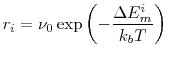
In this context, the rates in question are the oxygen vacancy migration rates. These migration events are thermally activated, with a migration rate given by [34]:
This code starts by reading in the system parameters from an input file. These values include things like simulation system dimensions, system temperature, number of steps to run, and particle populations, and are specified as key-value pairs (see Listing 4.1). A list is created for the particle objects, and for each particle, a random position initial position is generated such that the position falls on the required sublattice for that particle. Both the lattice type and sublattice types for each particle type are hard-coded, which presents a problem for generalization. If a new interacting particle is to be added to the system, the code must be modified and rebuilt so the input parsing routine can read the particle's population and so the initial position generator can tell which sublattice the particle should have a position on.
## kmc control input file
size_X	15
size_Y	15
size_Z	15
Temperature	1073
number_vacancy	0
number_hydrogen	0
number_IOx	34
monte_carlo_steps	500000
boltzmann	8.61738e-5
lattice	1
Listing 4.1: Original code configuration input file.
After the list of particles objects is created, the list of possible migration actions is read in from an input file. This includes the associated particle type/sublattice, attempt frequency, migration direction, and migration energy, and is specified in a multicolumn format (see Listing 4.2). When this data is read in, it is stored as a list of Action objects, which contain the specified information, as well as the migration rate for this action. Since these migration actions are assumed not to depend on the local configuration, once the action has been read it, all of the required information to calculate the migration rate from Equation 4.1 is known, so the migration rates are calculated and stored with the Action object. This presents a problem for generalization, as when the energy is allowed to depend on the local configuration, the migration rates could potentially change value at every time step for each particle in the system.
#[0]type [1]Entity [2]Sublattice [3]E [4]v0 [5-7] d[012]
migration  3  1  1.30  1e13  2  0  2
migration  3  1  1.30  1e13  2  0  -2
migration  3  1  1.30  1e13  2  2  0
migration  3  1  1.30  1e13  2  -2  0
migration  3  1  1.30  1e13  0  -2  2
migration  3  1  1.30  1e13  0  2  2
migration  3  1  1.30  1e13  0  -2  -2
migration  3  1  1.30  1e13  0  2  -2
migration  3  1  1.30  1e13  -2  0  2
migration  3  1  1.30  1e13  -2  0  -2
migration  3  1  1.30  1e13  -2  -2  0
migration  3  1  1.30  1e13  -2  2  0
Listing 4.2: Original code actions input
After both the Entity list and Action list have been initialized, the system is ready to be evolved. An event catalog of all of the possible migration events (step 2 of the general KMC algorithm in Section 4.1) is generated by scanning through the Entity list and Action list and checking each possible combination. For each combination of Entity and Action, a list of checks is performed to see if the pair is a valid migration event. This includes checking that the particle type that the action acts upon and the particle type of the paired Entity match and checking that the sublattice that the actions acts upon and the sublattice of the paired particle match. This is necessary as the lists can contain Entities and Actions for different particles on different sublattices, and it is important that the Entity and Actions selected for an Event are compatible (for example, attempting to apply an oxygen vacancy migration action on the fluorite tetrahedral interstitial sublattice to an oxygen interstitial on the fluorite octahedral interstitial sublattice would be a mistake). A check is also performed on the proposed final position of the particle to ensure that the final position is currently unoccupied (as moving a particle to a position where a particle already exists is not possible). As it will be shown later, this step, while necessary, is very computationally expensive because of the way the Entity objects are stored. If an Entity/Action pair passes all of the checks, it is considered a possible event, and Event object consisting of the Entity/Action pair is added to the event catalog.
Once the list of all possible events has been generated, a single event is chosen to be carried out. Since the migration energy for each event was assumed to be constant, the rates for all of these events are already known, so the partial sums of these rates are calculated and an event is randomly selected (steps 3-5 of the general KMC algorithm in Section 4.1). The event is carried out (step 6 of the general KMC algorithm in Section 4.1) by applying the Action to the Entity's position and updating the Entity object's internal position information. The simulation time is then updated using according to steps 8-9 of the general KMC algorithm in Section 4.1. At this point, the event catalog is no longer consistent with the system, so it is emptied in preparation for the next time step. The system loops over this process for the desired number of time steps.
Once the system has finished its evolution (i.e. the specified number of time steps have been carried out), the diffusion coefficient is calculated by:
Of primary concern was the handling of the particle positions. In the original code, while it was straightforward to get a specific particle's position, the reverse was not so straightforward. This caused a significant increase in computational complexity in the overall code run, specifically because of the Event validation checks. After a specific Entity and Action are confirmed to be a compatible pair, a check is performed to see if the final position after migration is already occupied. If it is occupied, the move is rejected, and if it is not, the move is accepted. Unfortunately, in the original code there is no direct way to resolve an Entity object from a given lattice position. Thus, in order to verify that a given position is unoccupied, the list of Entities must be scanned sequentially, with each each Entity's position compared to the position in question. If the position is indeed unoccupied, this method requires iteration of the entire list to confirm it as such. Because of this, the occupancy check is considered to have linear complexity with respect to the particle count. Since this check is performed while the event catalog is being constructed, which in itself is of linear complexity with respect to the particle count because each Entity must be checked against every Action, the construction of the Event catalog ends up being of quadratic complexity with respect to the particle count. Since the event catalog is reconstructed at each KMC time step, this quadratic complexity significantly impacts the overall performance of the code.
This quadratic complexity problem is addressed in the new KMC code by the addition of a bookkeeping data structure. As the code is written in C++, access to data structures' memory addresses (pointers) is permitted. With this capability available, what is essentially a map from 3-dimensional positions to Entity pointers is constructed. Since the code is Lattice Kinetic Monte Carlo, particles can only exist on specific lattice sites. As such, the lattice positions can be scaled in such a way as to make all the lattice coordinates non-negative integers. This allows the position map to be created as a list of lists of lists of Entity pointers. Since list access is constant time, this reduces the occupancy check complexity from linear to constant time with respect to particle count, which reduces the overall code complexity from quadratic to linear with respect to particle count. This structure is initialized as the particles are added to the Entity list at the beginning of the simulation, and with the constant time access can be easily updated after each migration event. This results in a huge performance gain compared to the original code, as simulations that would take hours in the original code could finish in minutes in the new code. This performance gain is shown explicitly in Section 5.1.
Since actions in the new code are allowed to have different energies based on the local environment, the data structures and the main algorithm need to be changed in the new code. The Event class is extended to hold a migration energy and migration rate, in addition to the references to the Entity and Action it is associated with. As the migration energy and migration rate are now associated with the Events in the event catalog, they need to be calculated each time the event catalog is populated. An additional step is added to the original code algorithm after the event catalog is populated to iterative over the events in the catalog and for each Event, determine the correct migration energy and calculate the corresponding migration rate.
In order to facilitate the generalization both to allow arbitrary particle types to be placed in the system and to allow arbitrarily complex local environments and corresponding energies to be specified, the systems for reading and writing data needs to be modified. In the original code, configuration entries were specified as key/value pairs (see Listing 4.1), while the action entries were specified in a multicolumn format (see Listing 4.2). These formats are sufficient for the simplified system the original code was designed for, but it is not sufficient for the complex interactions that need to be specified for this study. Attempting to use these simple tab-delimited formats for complex specifications would result in extremely complex input specifications and even more complex parsers and generators to write them. As I/O specification becomes more complicated it becomes very difficult to read/write input/output files without making mistakes. It also becomes more difficult to access these files programmatically, which makes both generating series of input files and analyzing the resulting output files more difficult.
This problem is solved by the introduction of XML as the method of data transport. XML schemas can be written for arbitrary data transport, which makes it ideal for customized data transport in custom codes such as this. The XML protocol is also very well supported, with XML interfaces either built into or readily available for almost every commonly used programming language. As such, it becomes almost trivial to read and write data from the program (e.g. instead of reading the system temperature from the output file by iterating down the lines of the file to the third line, then reading the fifth column of data or whatever, the entire data file can be automatically loaded into a data structure and the temperature can be obtained by some logical data structure accessors like $data->{config}->{temperature}).
Customized XML schemas for the various input and output files were developed, so input can be generated easily from any programming language with an XML module (almost every commonly used language). An additional input file for Entity naming and sublattice maps we also developed so that arbitrary particle types can be specified and properly added to the system without any modification of the code (see Listing 4.3), Also, when combined with bi-directional maps added to the code, this allows for logical particle names to be used in the input and output files instead of their internal numerical representation (e.g. the tetrahedral vacancy particle type can be represented by the logical name tet_vacancy instead of its internal numerical identifier ![]() ). The configuration input file specifies all of the system configuration parameters like the original code (see Listing 4.4). The actions input file specifies the information related to each migration action (see Listing 4.5), and is extended in the next section to support arbitrary local configuration dependent migration energies. Finally, the output file contains the calculated diffusion coefficient of each of the particles in the system, along with various runtime statistics (see Listing 4.6).
). The configuration input file specifies all of the system configuration parameters like the original code (see Listing 4.4). The actions input file specifies the information related to each migration action (see Listing 4.5), and is extended in the next section to support arbitrary local configuration dependent migration energies. Finally, the output file contains the calculated diffusion coefficient of each of the particles in the system, along with various runtime statistics (see Listing 4.6).
<?xml version="1.0" encoding="utf-8"?>
<entities>
  <entity>
    <name>sub_lanthanum</name>
    <sublattice>substitutional</sublattice>
  </entity>
  <entity>
    <name>tet_vacancy</name>
    <sublattice>tetrahedral</sublattice>
  </entity>
</entities>
Listing 4.3: Generalized code sample entities input
<?xml version="1.0" encoding="utf-8"?>
<configuration>
  <boltzmann_constant>8.61738e-5</boltzmann_constant>
  <dimensions>
    <x>15</x>
    <y>15</y>
    <z>15</z>
  </dimensions>
  <initial_populations>
    <population>
      <count>200</count>
      <entity>sub_lanthanum</entity>
    </population>
    <population>
      <count>100</count>
      <entity>tet_vacancy</entity>
    </population>
  </initial_populations>
  <lattice_parameter>5.411e-8</lattice_parameter>
  <lattice_type>face_centered_cubic</lattice_type>
  <simulation_steps>10000</simulation_steps>
  <temperature>1073</temperature>
</configuration>
Listing 4.4: Generalized code sample configuration input
<?xml version="1.0" encoding="utf-8"?>
<actions>
  <action>
    <direction>
      <x>0</x>
      <y>0</y>
      <z>2</z>
    </direction>
    <energy>0.7489</energy>
    <entity>tet_vacancy</entity>
    <frequency>1.0e13</frequency>
    <sublattice>tetrahedral</sublattice>
    <type>migration</type>
  </action>
  <action>
    <direction>
      <x>0</x>
      <y>0</y>
      <z>-2</z>
    </direction>
    <energy>0.7489</energy>
    <entity>tet_vacancy</entity>
    <frequency>1.0e13</frequency>
    <sublattice>tetrahedral</sublattice>
    <type>migration</type>
  </action>
  <action>
    <direction>
      <x>2</x>
      <y>0</y>
      <z>0</z>
    </direction>
    <energy>0.7489</energy>
    <entity>tet_vacancy</entity>
    <frequency>1.0e13</frequency>
    <sublattice>tetrahedral</sublattice>
    <type>migration</type>
  </action>
</actions>
Listing 4.5: Generalized code sample actions input (truncated to save space)
<?xml version="1.0" encoding="utf-8"?>
<results>
  <configuration>
    <temperature>1073</temperature>
    <lattice_type>face_centered_cubic</lattice_type>
    <lattice_parameter>5.411e-008</lattice_parameter>
    <dimensions>
      <x>15</x>
      <y>15</y>
      <z>15</z>
    </dimensions>
  </configuration>
  <entities>
    <entity>
      <name>sub_lanthanum</name>
      <initial_population>200</initial_population>
      <diffusivity>0</diffusivity>
      <square_displacement>0</square_displacement>
      <rms_displacement>0</rms_displacement>
    </entity>
    <entity>
      <name>tet_vacancy</name>
      <initial_population>100</initial_population>
      <diffusivity>8.821e-007</diffusivity>
      <square_displacement>1.570e-012</square_displacement>
      <rms_displacement>1.253e-007</rms_displacement>
    </entity>
  </entities>
  <time_series />
  <run_statistics>
    <run_time>552</run_time>
    <simulation_steps>10000</simulation_steps>
    <simulation_time>2.96782e-009</simulation_time>
    <average_time_step>2.96782e-013</average_time_step>
    <max_time_step>3.69887e-012</max_time_step>
    <min_time_step>2.8271e-017</min_time_step>
    <action_list_size>6</action_list_size>
    <arrangement_count>756</arrangement_count>
    <avg_event_catalog_size>520</avg_event_catalog_size>
    <max_event_catalog_size>594</max_event_catalog_size>
    <min_event_catalog_size>500</min_event_catalog_size>
  </run_statistics>
</results>
Listing 4.6: Generalized code sample output
Many different ideas were considered to implement this, but only one was sufficiently general to allow an arbitrary number of arbitrary configurations to be specified completely in the action input file without the need to modify or rebuild the code. This method is described here.
To begin, in a given local configuration (referred to as an Arrangement), each position to be considered is specified (referred to as a Restriction). A Restriction consists of a position/entity-type pair, where the position specifies the 3-dimensional position relative to the initial position of the migrating particle, and the entity-type is the type of Entity that should be present in that position. Each Arrangement contains an arbitrary length list of these Restrictions, along with the migration energy that corresponds to this set of Restrictions. An Arrangement can thus consider any arbitrary local configuration that is specified. The Action class is extended to contain an arbitrary length list of these Arrangements. Each Action can thus consider any number of arbitrary local configuration specified. For the local environment used in this study (Figure 3.1), there are 6 cation sites that influence the migration energy, so each Action contains 64 Arrangements corresponding to the 64 different possible configurations of the 6 cation sites, where each of these Arrangements contains 6 Restrictions that specify the positions and entity-types of the configuration, along with the migration energy that correspond to that configuration. A sample Action containing a local arrangement is shown in Listing 4.7 (note that since only the defects are simulated, not the background CeO![]() lattice, an ``empty'' cation site corresponds to a Ce atom). Constructing such an action file can be quite daunting if done manually, but since it is written in XML, it can be constructed logically in a programming language data structure and then exported to XML using the language's XML interface.
lattice, an ``empty'' cation site corresponds to a Ce atom). Constructing such an action file can be quite daunting if done manually, but since it is written in XML, it can be constructed logically in a programming language data structure and then exported to XML using the language's XML interface.
After this information is loaded into the Action data structure, it can be used during the migration rate calculation step discussed in Section 4.3.2. During this step, rather than just taking the migration base migration energy specified in the action file, the code first checks the associated Arrangements to see if any of them apply. It does this by iterating over the list of Arrangements sequentially, and using the energy associated with the first Arrangement that applies to the event. It checks each Arrangement by iterating over the list of Restrictions for the Arrangement and checking the positions and entity types specified by these Restrictions. If any of the Restrictions do not match, the Arrangement does not apply to the Event, and if all of the Restrictions match, the Arrangement does apply to the Even. If after checking all of the Arrangements none of them are found to match, the base migration energy (this can thought of as the ``default'' energy) for the Action is used. Once the migration energy has been determined, the migration rate is calculated in the normal way from Equation 4.1.
<?xml version="1.0" encoding="utf-8"?>
<actions>
  <action>
    <arrangements>
      <arrangement>
        <energy>0.5366</energy>
        <restrictions>
          <restriction>
            <direction>
              <x>-1</x>
              <y>1</y>
              <z>-1</z>
            </direction>
            <entity>no_entity</entity>
          </restriction>
          <restriction>
            <direction>
              <x>1</x>
              <y>-1</y>
              <z>-1</z>
            </direction>
            <entity>sub_lanthanum</entity>
          </restriction>
          <restriction>
            <direction>
              <x>-1</x>
              <y>-1</y>
              <z>1</z>
            </direction>
            <entity>no_entity</entity>
          </restriction>
        </restrictions>
      </arrangement>
    </arrangements>
    <direction>
      <x>0</x>
      <y>0</y>
      <z>2</z>
    </direction>
    <energy>0.7489</energy>
    <entity>tet_vacancy</entity>
    <frequency>1.0e13</frequency>
    <sublattice>tetrahedral</sublattice>
    <type>migration</type>
  </action>
</actions>
Listing 4.7: Generalized code sample action with arrangement