Results and Discussion

Computational Complexity

As was discussed in Section 4.3.1, because of the way positions are stored in the original code there is no direct way to resolve a lattice position to a particle, which results in quadratic complexity with respect to the particle count. This is solved in the generalized code by the introduction of a position-entity map, which reduces position lookups to constant time, and overall code complexity to linear time. To demonstrate this, the generalized code is used to run the same simulation environment that the original code is capable of running. This is a fluorite UO$_2$ lattice with interstitial oxygen atoms added in various concentrations to study hyperstoichiometric effects. The migration energy and attempt frequency are taken to be the same as what was provided with the original code ($E_m = 1.1$ eV, $\nu_0 = 1 \times 10^{13}$ Hz). 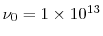The simulation system was taken to be a $15 \times 15 \times 15$ unit cell cubic system with periodic boundary conditions. The runtime results for these simulations are provided in a linear scale in Figure 5.1 to show the complexity trends, and in a logarithmic scale in Figure 5.2 for a more useful comparison of the actual time values. These results show the enormous improvement in complexity and runtime, which is critical to the performance of the local configuration-dependent simulations. Without this improvement this improvement the more complex simulations would extraordinary long times to complete.

Figure 5.1: Comparison of computational complexity with respect to the particle count (show here as a function of the stoichiometric parameter) shown on a linear scale to demonstrate complexity trends. Here ``Inefficient'' refers to the original code algorithm, while ``Efficient'' refers to the generalized code algorithm.

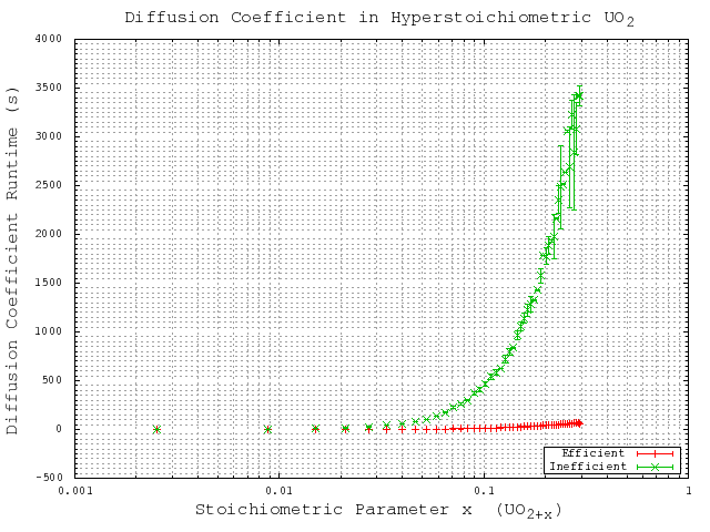Figure 5.2: Comparison of computational complexity with respect to the particle count (show here as a function of the stoichiometric parameter) shown on a logarithmic scale for accurate comparison of runtime values. Here ``Inefficient'' refers to the original code algorithm, while ``Efficient'' refers to the generalized code algorithm.

Code Verification

First, it is important to verify that the generalized code is able to reproduce the results of the original code, to confirm that the core functionality of the generalized code is consistent with that of the original code. To confirm this, the diffusivity results from the computation complexity simulations are compared. These simulations provided the oxygen interstitial diffusion coefficient $D_i$ from Equation (4.2). The oxygen self-diffusivity is then calculated by:

$$D_O = [O_i'']D_i$$ (5.1)

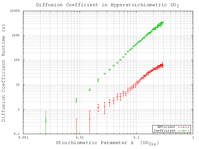
where $D_O$ is the oxygen self-diffusivity, $[O_i'']$ is the oxygen interstitial mole fraction, and $D_i$ is the oxygen interstitial diffusivity. The computed results from the original code and from the generalized code are compared with each other, and with experimentally measures values provided by Contamin [35] and Murch [36]. The results are given in Figure 5.3. These results show excellent agreement between the calculated results from the original code and generalized code, and between the calculated results and the experimentally measured values.

Figure 5.3: Comparison of calculated and experimentally measured oxygen self-diffusivities in hyperstoichoimetric UO$_2$. Here ``Inefficient'' refers to the original code algorithm, while ``Efficient'' refers to the generalized code algorithm.

With the core functionality verified, it is also important to verify the most important extension to the original code: the local configuration depedent energies. The code to read the complex XML input data and store it in the Action data structures, as well as the code to scan for these configurations during migration energy determination is quite extensive. It is important confirm that these configurations are being recognized correctly by the code as it checks through them. To verify this, the code was modified to output the configuration found as it scans through the local environment of each particle. These counts were aggregated for several different non-stoichiometric values $x$ in $La_{x}Ce_{1-x}O_{2-x/2}$. 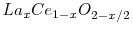The distribution of these configuration changes according to the energies, to confirm the expected initial random distributions, only the configurations for the initial time step are considered. These results are given in Figure 5.4. The configuration number in these figures corresponds to the row number of the configuration at specified in Table 3.2, and can be thought of as increasing with increasing number of neighbor lanthanum cations. These results show that as expected, for low dopant concentrations the configurations found are concentrated around the 0-1 neighbor lanthanum cation configurations, and as the dopant concentration increases, the configuration distribution spreads out to include the higher neighbor lanthanum cation configurations.

Figure 5.4: Configuration distribution verification for initial configurations at increasing non-stoichiometries. The configuration number corresponds to the row number of the configuration at specified in Table 3.2.

Potential Validation

To analyze the validity of the potentials described in Table 2.1, KMC simulations are performed using the local configuration dependent migrations energies calculated from these potentials. These simulations are performed on a fluorite UO$_2$ lattice with lanthanum added to the system in various concentrations to study hypostoichiometric effects. The simulation system was taken to be a $15 \times 15 \times 15$ unit cell cubic system with periodic boundary conditions at $800 \ensuremath{\,^{\circ}\mathrm{C}}$. 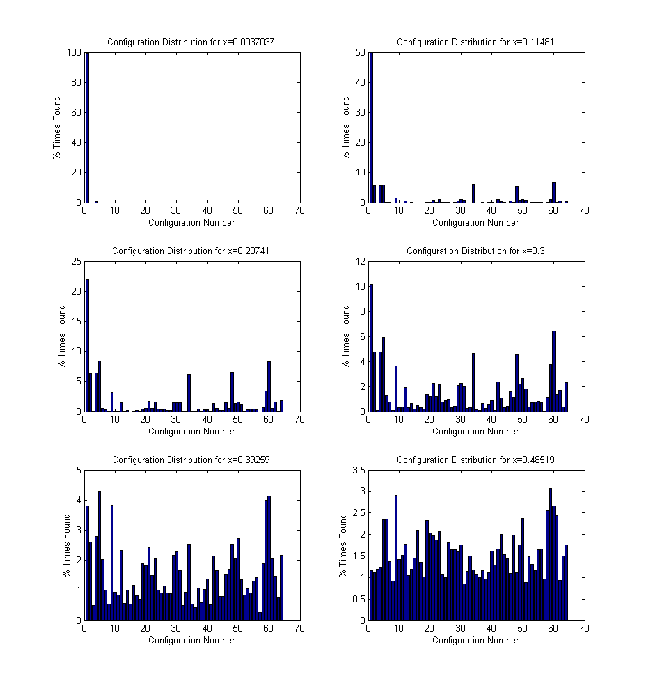Oxygen tetrahedral vacancies and lanthanum substitutional atoms are added according to the vacancy compensation mechanism in Equation 2.4. The local configuration depenent vacancy migration energies for each potential are taken from Table 3.2. To be sure that the event catalog and migration energies are properly sampled, it is important to select a sufficiently large number of simulations steps to run, especially for high dopant concentrations. In order to ensure that a sufficiently large number of steps is used in the validation study, the simulations for one of the potentials were run with increasing simulation steps until the solutions converged. The results are shown in Figure 5.5, and indicate that $500,000$ KMC steps is sufficient to get converged results for this system. While this study was only performed for one potential (Gotte [22]), it is assumed that the conclusion can be transfered to the other potentials since the simulations for these potentials use the same particle concentrations and configurational complexity.

Figure 5.5: KMC simulation steps comparison using migration energies derived from the Gotte [22] potential.

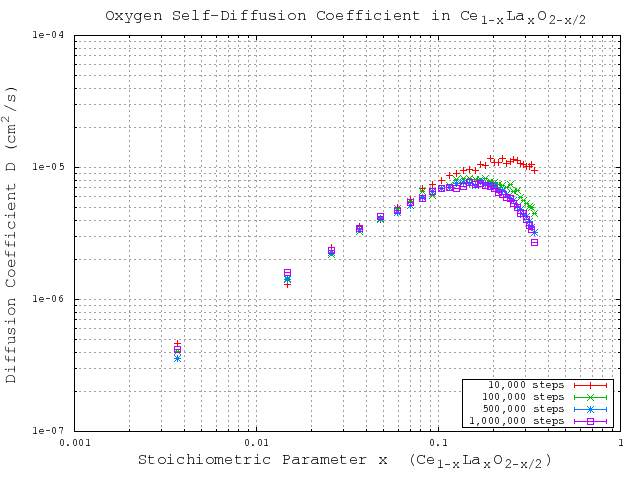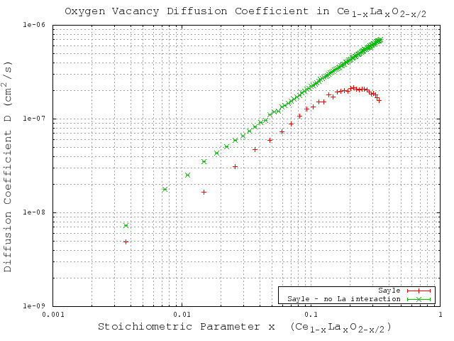
With the sufficiently large number of KMC steps determined, the KMC simulations for varying dopant concentrations are performed using the migration energies derived for each of the three potentials (Table 3.2). The same simulations are performed using a constant migration energy that corresponds to the case of zero neighbor lanthanum cations (pure hypostoichiometric ceria) in order to demonstrate the effect of the lanthanum interactions. The results of these simulations are given in Figure 5.7 (Gotte [22]), Figure 5.8 (Minervini [7]), and Figure 5.9 (Sayle [23]). Diffusivity results from all three potentials clearly show the desired lanthanum trapping effect, so in this sense they are all reasonable potentials. However, each potential shows peak oxygen diffusivity at different dopant concentrations. To see which produces the most realistic result, the peak diffusivities are compared to experimental results by Faber et. al [37]. Faber et al. studied ionic conductivity in ceria doped with several different dopant species. From the ionic conductivity, they calculated the effective activation energy for diffusion. The calculated values for lanthanum doped ceria are shown in Figure 5.6. The overall effective activation energy essentially determines how easy it is for ions to diffuse, so from this it is inferred that the minimum overall activation energy should roughly correspond to the peak oxygen diffusivity. The minimum activation energy as found by Faber occurs at around 5% lanthanum concentration, while the peak diffusivities from Gotte, Minervini, and Sayle occur around 12%, 20%, and 23% respectively. Based on these results, it is concluded that out of the three, the Gotte potential yielded the most realistic diffusion curve.

Figure 5.6: Effective activation energy as a function of non-stoichiometry in La-doped ceria [37].

Figure 5.7: KMC simulation results for migration energies derived from the Gotte [22] potential.

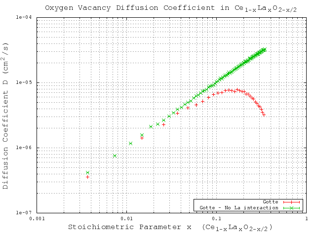Figure 5.8: KMC simulation results for migration energies derived from the Minervini [7] potential.

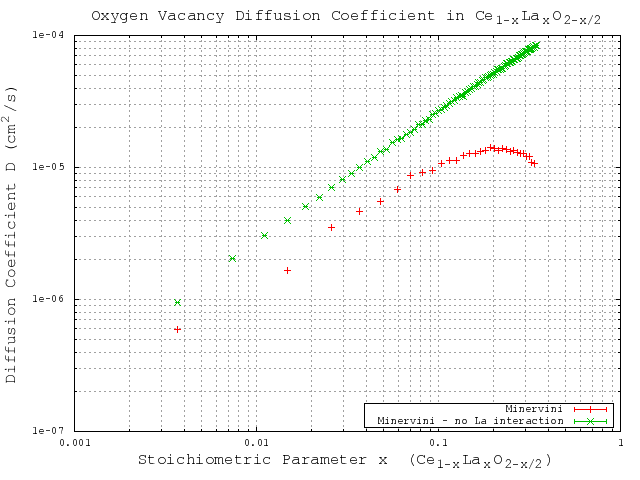Figure 5.9: KMC simulation results for migration energies derived from the Sayle [23] potential.